
Dynamic Workload Driven Data Integration in Tableau
Kristi Morton
∗
University of Washington
kmorton@cs.washington.edu
Ross Bunker, Jock Mackinlay, Robert
Morton, and Chris Stolte
Tableau Software
{
rbunker,jmackinlay,rmorton,cstolte}@tableausoftware.com
ABSTRACT
Tableau
is
a
commercial
business
intelligence
(BI)
software
tool that supports interactive, visual analysis of data.
Armed
with
a
visual
interface
to
data
and
a
focus
on
usability,
Tableau enables a wide audience of end-users to gain insight
into
their
datasets.
The
user
experience
is
a
fluid
process
of
interaction in which exploring and visualizing data takes just
a
few
simple
drag-and-drop
operations
(no
programming
or
DB
experience
necessary).
In
this
context
of
exploratory,
ad-hoc visual analysis,
we describe a novel approach to inte-
grating large, heterogeneous data sources.
We present a new
feature
in
Tableau
called
data
blending
,
which
gives
users
the
ability
to
create
data
visualization
mashups
from
struc-
tured,
heterogeneous
data
sources
dynamically
without
any
upfront
integration
effort.
Users
can
author
visualizations
that
automatically
integrate
data
from
a
variety
of
sources,
including
data
warehouses,
data
marts,
text
files,
spread-
sheets,
and
data
cubes.
Because
our
data
blending
system
is
workload
driven,
we
are
able
to
bypass
many
of
the
pain-
points
and
uncertainty
in
creating
mediated
schemas
and
schema-mappings
in
current
pay-as-you-go
integration
sys-
tems.
Categories
and
Subject
Descriptors:
H.5.0
[Informa-
tion
Systems]:
Information
Interfaces
and
Presentation
General
Terms:
Design,
Human
Factors,
Management
Keywords:
Data
Integration,
Visualization
1.
INTRODUCTION
Unlike
databases,
human
brains
have
limited
capacity
for
managing
and
making
sense
of
large
collections
of
data.
In
database
terms,
the
feat
of
gaining
insight
in
big
data
is
of-
ten
accomplished
by
issuing
aggregation
and
filter
queries.
Yet, this approach is time-consuming as the user is forced to
∗
Work
done
as
intern
at
Tableau
Software,
Seattle.
Permission
to
make
digital
or
hard
copies
of
all
or
part
of
this
work
for
personal
or
classroom
use
is
granted
without
fee
provided
that
copies
are
not made or distributed for profit or commercial advantage and that copies
bear this notice and the full citation on the first page.
To copy otherwise, to
republish, to post on servers or to redistribute to lists, requires prior specific
permission and/or a fee.
SIGMOD ‘12,
May 20–24, 2012, Scottsdale, Arizona, USA.
Copyright 2012 ACM 978-1-4503-1247-9/12/05 ...$10.00.
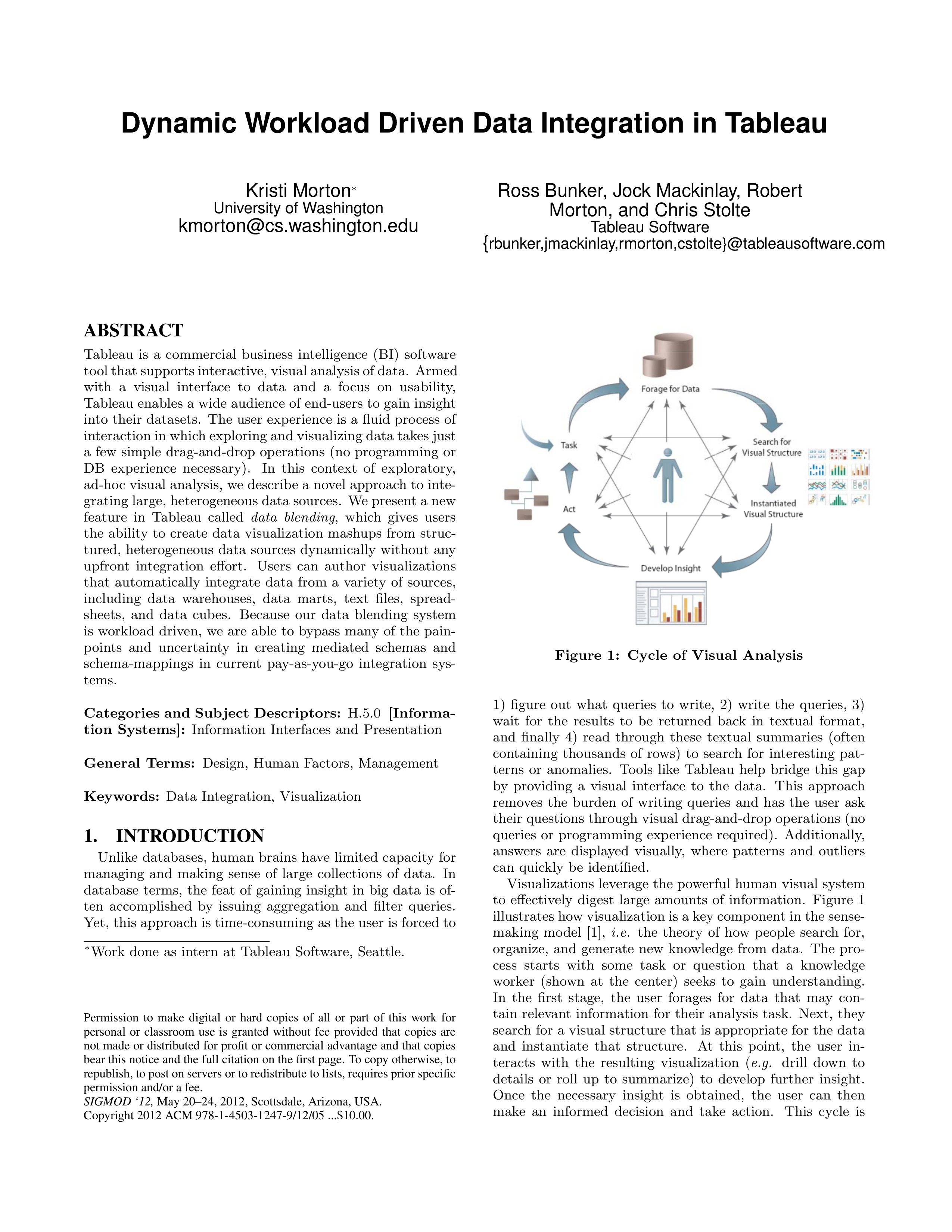
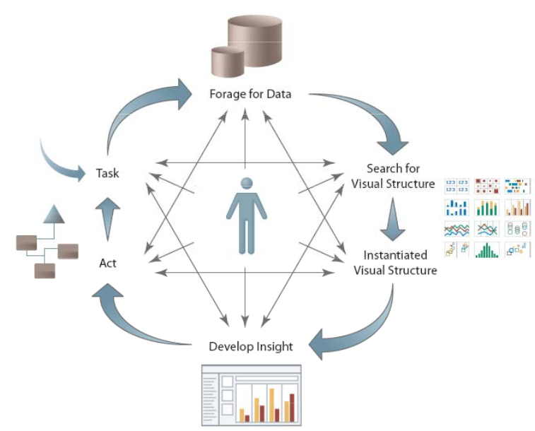
Figure
1:
Cycle
of
Visual
Analysis
1)
figure
out
what
queries
to
write,
2)
write
the
queries,
3)
wait
for
the
results
to
be
returned
back
in
textual
format,
and
finally
4)
read
through
these
textual
summaries
(often
containing
thousands
of
rows)
to
search
for
interesting
pat-
terns
or
anomalies.
Tools
like
Tableau
help
bridge
this
gap
by
providing
a
visual
interface
to
the
data.
This
approach
removes
the
burden
of
writing
queries
and
has
the
user
ask
their questions through visual drag-and-drop operations (no
queries
or
programming
experience
required).
Additionally,
answers
are
displayed
visually,
where
patterns
and
outliers
can
quickly
be
identified.
Visualizations
leverage
the
powerful
human
visual
system
to
effectively
digest
large
amounts
of
information.
Figure
1
illustrates how visualization is a key component in the sense-
making
model
[1],
i.e.
the
theory
of
how
people
search
for,
organize,
and
generate
new
knowledge
from
data.
The
pro-
cess
starts
with
some
task
or
question
that
a
knowledge
worker
(shown
at
the
center)
seeks
to
gain
understanding.
In
the
first
stage,
the
user
forages
for
data
that
may
con-
tain
relevant
information
for
their
analysis
task.
Next,
they
search
for
a
visual
structure
that
is
appropriate
for
the
data
and
instantiate
that
structure.
At
this
point,
the
user
in-
teracts
with
the
resulting
visualization
(
e.g.
drill
down
to
details
or
roll
up
to
summarize)
to
develop
further
insight.
Once
the
necessary
insight
is
obtained,
the
user
can
then
make
an
informed
decision
and
take
action.
This
cycle
is
centered
around
and
driven
by
the
user
and
requires
that
the
visualization
system
be
flexible
enough
to
support
user
feedback
and
allow
alternative
paths
based
on
the
needs
of
the
user’s
exploratory
tasks.
Most
visualization
tools
[4,
5,
13],
however,
treat
this
cycle
as
a
single,
directed
pipeline,
and
offer
limited
interaction
with
the
user.
Moreover,
users
often
want
to
ask
their
analytical
ques-
tions
over
multiple
data
sources.
However,
the
task
of
set-
ting up data for integration is orthogonal to the analysis task
at
hand,
requiring
a
context
switch
that
interrupts
the
nat-
ural flow of the analysis cycle.
We extend the visual analysis
cycle with a new feature called
data
blending
that allows the
user
to
seamlessly
combine
and
visualize
data
from
multiple
different data sources on-the-fly.
Our blending system issues
live
queries
to
each
data
source
to
extract
the
minimum
in-
formation
necessary
to
accomplish
the
visual
analysis
task.
Often,
the
visual
level
of
detail
is
at
a
coarser
level
than
the
data
sets.
Aggregation
queries,
therefore,
are
issued
to
each
data
source
before
the
results
are
copied
over
and
joined
in
Tableau’s
local
in-memory
view.
We
refer
to
this
type
of
join
as
a
post-aggregate
join
and
find
it
a
natural
fit
for
ex-
ploratory
analysis,
as
less
data
is
moved
from
the
sources
for
each
analytical
task,
resulting
in
a
more
responsive
sys-
tem.
Finally,
Tableau’s
data
blending
feature
automatically
infers
how
to
integrate
the
datasets
on-the-fly,
involving
the
user
only
in
resolving
conflicts.
This
system
also
addresses
a
few
other
key
data
integration
challenges,
including
com-
bining
datasets
with
mismatched
domains
or
different
levels
of
detail
and
dirty
or
missing
data
values.
One
interesting
property
of
blending
data
in
the
context
of
a
visualization
is
that
the
user
can
immediately
observe
any
anomalies
or
problems
through
the
resulting
visualization.
These
aforementioned
design
decisions
were
grounded
in
the
needs
of
Tableau’s
typical
BI
user
base.
Thanks
to
the
availability
of
a
wide-variety
of
rich
public
datasets
from
sites
like
data.gov,
many
of
Tableau’s
users
integrate
data
from
external
sources
such
as
the
Web
or
corporate
data
such
as
internally-curated
Excel
spreadsheets
into
their
en-
terprise
data
warehouses
to
do
predictive,
what-if
analysis.
However,
the
task
of
integrating
external
data
sources
into
their
enterprise
systems
is
complicated.
First,
such
reposi-
tories
are
under
strict
management
by
IT
departments,
and
often
IT
does
not
have
the
bandwidth
to
incorporate
and
maintain
each
additional
data
source.
Second,
users
often
have
restricted
permissions
and
cannot
add
external
data
sources
themselves.
Such
users
cannot
integrate
their
exter-
nal
and
enterprise
sources
without
having
them
collocated.
An
alternative
approach
is
to
move
the
data
sets
to
a
data
repository that the user has access to, but moving large data
is
expensive
and
often
untenable.
We
therefore
architected
data blending with the following principles in mind:
1) move
as
little
data
as
possible,
2)
push
the
computations
to
the
data, and 3) automate the integration challenges as much as
possible,
involving
the
user
only
in
resolving
conflicts.
The
rest
of
this
paper
is
organized
as
follows.
First
in
Section
2
we
present
a
brief
overview
of
Tableau
and
data
blending.
Then
in
Section
3
we
discuss
the
use-case
scenar-
ios
and
underlying
principles
that
drove
the
design
of
our
data
blending
architecture.
Section
4
describes
our
overall
approach
to
data
blending.
Section
5
covers
related
work.
Finally,
in
Section
6,
we
discuss
interesting
research
direc-
tions,
and
in
Section
7
we
conclude.
!"#$%&'("&()**
+,-(./&(01.2%1(2$(3**
)4561$27%1$
898*:;<:8==
)?5/&21
8@9:>*A<AA89B<B
)$5"?1
>=:*<;<=:B;C=
!"#$%&'("&
)&*+
,$-+$%(."&%+/0%'(&+%*(
1*&(2333(/04*(50&%67
)-86+$07%+$
29:
)/8*&0+
93
)$8"/+
2;<
Primary Data Table
!"#$%&'("&()**
+",#-.%/"$
)012.$/3%.$
45675869:;
)-1<&/.
=865==694>
)$1"-.
:=674;6=>=
Secondary Data Table A
Secondary Data Table B
!"#$%&'("&
)&*+
,$-+$%
."&%+/0%'
&+%*(1*&(233
4"1#/+%0"$
564(1*&(7+10%+(0$(
896
)-:;+$0<%+$
2=>
?@AB@CA>2D
2E23B>@B2FF@D
)/:*&0+
=C
FCA@FFA>?E
2AEBD3C@CC2E?@?
)$:"/+
2?D
2FAB?DAFEF
DFB3@>@FB?>=F
Blended Data Table
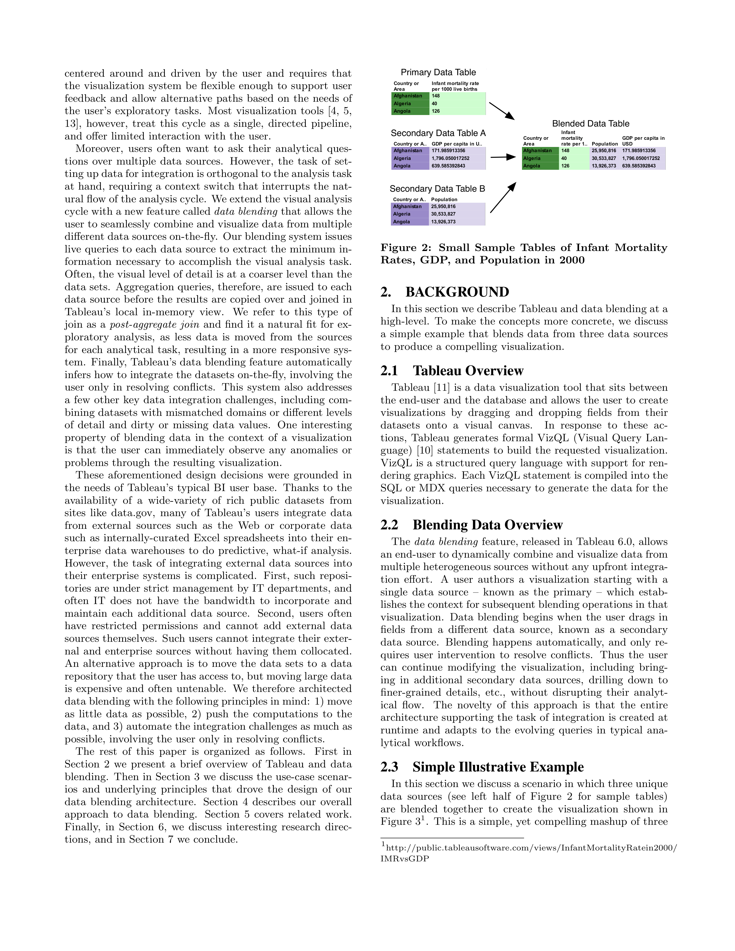
Figure
2:
Small
Sample
Tables
of
Infant
Mortality
Rates,
GDP,
and
Population
in
2000
2.
BACKGROUND
In this section we describe Tableau and data blending at a
high-level.
To
make
the
concepts
more
concrete,
we
discuss
a
simple
example
that
blends
data
from
three
data
sources
to
produce
a
compelling
visualization.
2.1
Tableau Overview
Tableau
[11]
is
a
data
visualization
tool
that
sits
between
the
end-user
and
the
database
and
allows
the
user
to
create
visualizations
by
dragging
and
dropping
fields
from
their
datasets
onto
a
visual
canvas.
In
response
to
these
ac-
tions,
Tableau
generates
formal
VizQL
(Visual
Query
Lan-
guage)
[10]
statements
to
build
the
requested
visualization.
VizQL
is
a
structured
query
language
with
support
for
ren-
dering graphics.
Each VizQL statement is compiled into the
SQL
or
MDX
queries
necessary
to
generate
the
data
for
the
visualization.
2.2
Blending Data Overview
The
data
blending
feature,
released
in
Tableau
6.0,
allows
an end-user to dynamically combine and visualize data from
multiple heterogeneous sources without any upfront integra-
tion
effort.
A
user
authors
a
visualization
starting
with
a
single
data
source
–
known
as
the
primary
–
which
estab-
lishes the context for subsequent blending operations in that
visualization.
Data
blending
begins
when
the
user
drags
in
fields
from
a
different
data
source,
known
as
a
secondary
data
source.
Blending
happens
automatically,
and
only
re-
quires
user
intervention
to
resolve
conflicts.
Thus
the
user
can
continue
modifying
the
visualization,
including
bring-
ing
in
additional
secondary
data
sources,
drilling
down
to
finer-grained
details,
etc.,
without
disrupting
their
analyt-
ical
flow.
The
novelty
of
this
approach
is
that
the
entire
architecture
supporting
the
task
of
integration
is
created
at
runtime
and
adapts
to
the
evolving
queries
in
typical
ana-
lytical
workflows.
2.3
Simple Illustrative Example
In this section we discuss a scenario in which three unique
data
sources
(see
left
half
of
Figure
2
for
sample
tables)
are
blended
together
to
create
the
visualization
shown
in
Figure
3
1
.
This
is
a
simple,
yet
compelling
mashup
of
three
1
http://public.tableausoftware.com/views/InfantMortalityRatein2000/
IMRvsGDP
!""
!#"""
!"#"""
!""#"""
$
%
&
!'
($
'%
!$&
$)'
!"#$%&
'$($%)
*
+"&#(
,-
./#"(
01
'23$/
456#7(
89
.3:(
*
'(3&#
46(:#(
;1
<%=#72
;;
>6(?#@
;-
A(B("
0
45C/("#)$("
D9-
E36F%G
0,
4"C2@(
D;,
.?%7/HI%B3:@#7
9
J$/#2B#
KD
<G("L(6
,0
'M%&%"
0
'#"C(B26%
0
!"#$"%&'()%$*+%,&)$%-&.-)&/000&*+1-&2+)%34
!"#$%&'$()%*+)$*,$-."
!"#$%&'(")
!"#$%"&##
'##"###"###
("###"###"###
("$)$")!'"###
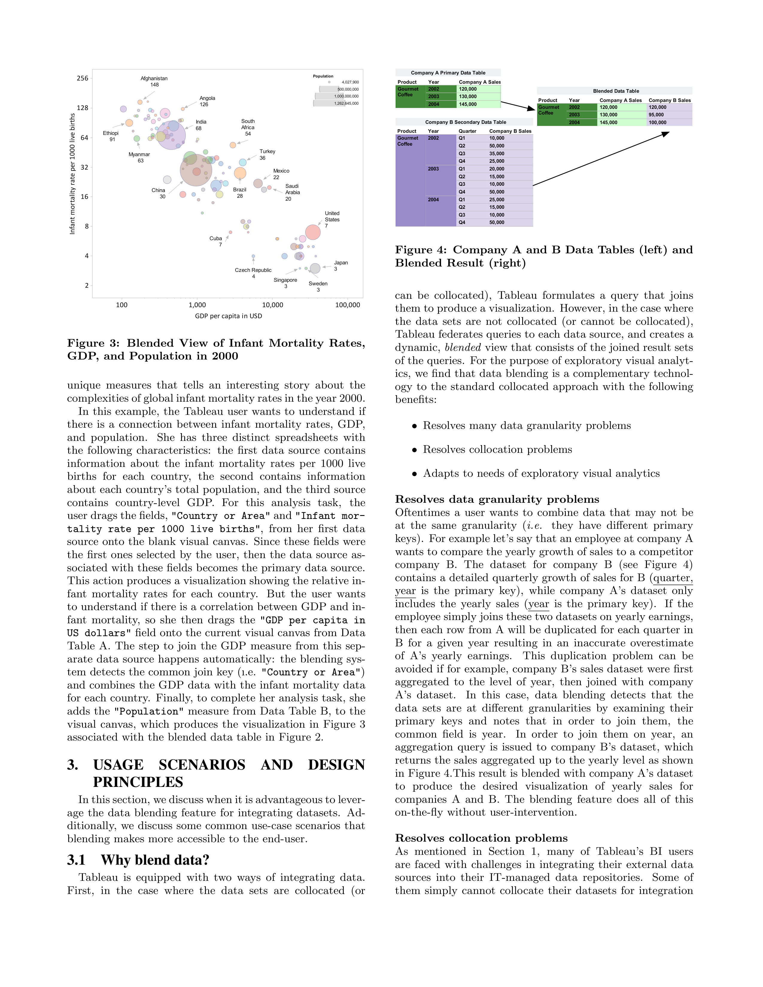
Figure
3:
Blended
View
of
Infant
Mortality
Rates,
GDP,
and
Population
in
2000
unique
measures
that
tells
an
interesting
story
about
the
complexities of global infant mortality rates in the year 2000.
In
this
example,
the
Tableau
user
wants
to
understand
if
there
is
a
connection
between
infant
mortality
rates,
GDP,
and
population.
She
has
three
distinct
spreadsheets
with
the
following
characteristics:
the
first
data
source
contains
information
about
the
infant
mortality
rates
per
1000
live
births
for
each
country,
the
second
contains
information
about
each
country’s
total
population,
and
the
third
source
contains
country-level
GDP.
For
this
analysis
task,
the
user drags the fields,
"Country
or
Area"
and
"Infant
mor-
tality
rate
per
1000
live
births"
,
from
her
first
data
source
onto
the
blank
visual
canvas.
Since
these
fields
were
the
first
ones
selected
by
the
user,
then
the
data
source
as-
sociated
with
these
fields
becomes
the
primary
data
source.
This action produces a visualization showing the relative in-
fant
mortality
rates
for
each
country.
But
the
user
wants
to
understand
if
there
is
a
correlation
between
GDP
and
in-
fant
mortality,
so
she
then
drags
the
"GDP
per
capita
in
US
dollars"
field
onto
the
current
visual
canvas
from
Data
Table
A.
The
step
to
join
the
GDP
measure
from
this
sep-
arate
data
source
happens
automatically:
the
blending
sys-
tem
detects
the
common
join
key
(ı.e.
"Country
or
Area"
)
and
combines
the
GDP
data
with
the
infant
mortality
data
for
each
country.
Finally,
to
complete
her
analysis
task,
she
adds
the
"Population"
measure
from
Data
Table
B,
to
the
visual
canvas,
which
produces
the
visualization
in
Figure
3
associated
with
the
blended
data
table
in
Figure
2.
3.
USAGE
SCENARIOS
AND
DESIGN
PRINCIPLES
In this section, we discuss when it is advantageous to lever-
age
the
data
blending
feature
for
integrating
datasets.
Ad-
ditionally,
we
discuss
some
common
use-case
scenarios
that
blending
makes
more
accessible
to
the
end-user.
3.1
Why blend data?
Tableau
is
equipped
with
two
ways
of
integrating
data.
First,
in
the
case
where
the
data
sets
are
collocated
(or
!"#$%&'
()*"
+%*"')"
,#-.*/01213*4)5
6#%"-)'
,#77))
8998
+:
:9;999
+8
<9;999
+=
=<;999
+>
8<;999
899=
+:
89;999
+8
:<;999
+=
:9;999
+>
<9;999
899>
+:
8<;999
+8
:<;999
+=
:9;999
+>
<9;999
,#-.*/01213)&#/$*"01?*'*1@*A4)
!"#$%&'
()*"
+#,-*./0102*3)4
5#%",)'
+#66))
7887
978:888
788;
9;8:888
788<
9<=:888
+#,-*./010!">,*"/0?*'*0@*A3)
!"#$%&'
()*"
+#,-*./0102*3)4
+#,-*./0502*3)4
6#%",)'
+#77))
8998
:89;999
:89;999
899<
:<9;999
=>;999
899?
:?>;999
:99;999
53).$)$0@*'*0A*B3)
Figure
4:
Company
A
and
B
Data
Tables
(left)
and
Blended
Result
(right)
can
be
collocated),
Tableau
formulates
a
query
that
joins
them to produce a visualization.
However, in the case where
the
data
sets
are
not
collocated
(or
cannot
be
collocated),
Tableau
federates
queries
to
each
data
source,
and
creates
a
dynamic,
blended
view
that
consists
of
the
joined
result
sets
of the queries.
For the purpose of exploratory visual analyt-
ics,
we
find
that
data
blending
is
a
complementary
technol-
ogy
to
the
standard
collocated
approach
with
the
following
benefits:
•
Resolves
many
data
granularity
problems
•
Resolves
collocation
problems
•
Adapts
to
needs
of
exploratory
visual
analytics
Resolves
data
granularity
problems
Oftentimes
a
user
wants
to
combine
data
that
may
not
be
at
the
same
granularity
(
i.e.
they
have
different
primary
keys).
For example let’s say that an employee at company A
wants to compare the yearly growth of sales to a competitor
company
B.
The
dataset
for
company
B
(see
Figure
4)
contains
a
detailed
quarterly
growth
of
sales
for
B
(quarter,
year
is
the
primary
key),
while
company
A’s
dataset
only
includes
the
yearly
sales
(year
is
the
primary
key).
If
the
employee simply joins these two datasets on yearly earnings,
then
each
row
from
A
will
be
duplicated
for
each
quarter
in
B
for
a
given
year
resulting
in
an
inaccurate
overestimate
of
A’s
yearly
earnings.
This
duplication
problem
can
be
avoided
if
for
example,
company
B’s
sales
dataset
were
first
aggregated
to
the
level
of
year,
then
joined
with
company
A’s
dataset.
In
this
case,
data
blending
detects
that
the
data
sets
are
at
different
granularities
by
examining
their
primary
keys
and
notes
that
in
order
to
join
them,
the
common
field
is
year.
In
order
to
join
them
on
year,
an
aggregation
query
is
issued
to
company
B’s
dataset,
which
returns
the
sales
aggregated
up
to
the
yearly
level
as
shown
in
Figure
4.This
result
is
blended
with
company
A’s
dataset
to
produce
the
desired
visualization
of
yearly
sales
for
companies
A
and
B.
The
blending
feature
does
all
of
this
on-the-fly
without
user-intervention.
Resolves
collocation
problems
As
mentioned
in
Section
1,
many
of
Tableau’s
BI
users
are
faced
with
challenges
in
integrating
their
external
data
sources
into
their
IT-managed
data
repositories.
Some
of
them
simply
cannot
collocate
their
datasets
for
integration
!"##$%&'%()*
!""#
$%&'()*+,&-.
!"#$%&'
!"#$%&'()*'&)+,-'()./,/0$)
1'&/#$#/23
()#$%&'
4#1')'5*'6/0(62).2'0&73
*+,+-.'
!,(/#('(/
!"#$%&'#()'&"#$%&'*+'(#%,*(-.'#'/#01,()"2'%2,34%"
!"#$%$&'$()*+(,%-,$*./0
1
21
31
41
51
61
71
81
91
:;"?@$+%-)?)*<%#$.)"<"),0
1
2
3
4
5
6
7
8
9
A
!""#
!"#$%
&'(')*
*''('''('''
+('''('''('''
+(),-(.*-(+/)
0123$45627289
:;$9"6<
=5:3"<5?5@<6"A"6
=892B$5?50$4>9<75:3CC
D"EE7$5=5?5F29>1CC
!28>15:3"<
!8GH!<1<9<45:A9"6<
BC/)."*
BC/).*<"*
B.CD*
B.@$+"*
B.E$+)"+*
B+E?<*
B<E$."*
B<D*+"*
F<*+=
B#E;*+"/)*+
07"6I59J%
!$'0&)"#8"$#8"/7
!$'0&)"#8"$#8"/7
!$'0&)"#8"$#8"/7
!$'0&)"#8"$#8"/7
!$'0&)"#8"$#8"/7
!$'0&)"#8"$#8"/7
!$'0&)"#8"$#8"/7
!$'0&)"#8"$#8"/7
!$'0&)"#8"$#8"/7
!$'0&)"#8"$#8"/7
!$'0&)"#8"$#8"/7
!$'0&)"#8"$#8"/7
!$'0&)"#8"$#8"/7
!$'0&)"#8"$#8"/7
!$'0&)"#8"$#8"/7
!$'0&)"#8"$#8"/7
!$'0&)"#8"$#8"/7
!$'0&)"#8"$#8"/7
!$'0&)"#8"$#8"/7
!$'0&)"#8"$#8"/7
!$'0&)"#8"$#8"/7
!$'0&)"#8"$#8"/7
!$'0&)"#8"$#8"/7
!$'0&)"#8"$#8"/7
!$'0&)"#8"$#8"/7
!$'0&)"#8"$#8"/7
!$'0&)"#8"$#8"/7
!$'0&)"#8"$#8"/7
!$'0&)"#8"$#8"/7
!$'0&)"#8"$#8"/7
!$'0&)"#8"$#8"/7
!$'0&)"#8"$#8"/7
!$'0&)"#8"$#8"/7
!$'0&)"#8"$#8"/7
!$'0&)"#8"$#8"/7
!$'0&)"#8"$#8"/7
!$'0&)"#8"$#8"/7
!$'0&)"#8"$#8"/7
!$'0&)"#8"$#8"/7
!$'0&)"#8"$#8"/7
!$'0&)"#8"$#8"/7
!$'0&)"#8"$#8"/7
!$'0&)"#8"$#8"/7
!$'0&)"#8"$#8"/7
!$'0&)"#8"$#8"/7
!$'0&)"#8"$#8"/7
!$'0&)"#8"$#8"/7
!$'0&)"#8"$#8"/7
!$'0&)"#8"$#8"/7
!$'0&)"#8"$#8"/7
!$'0&)"#8"$#8"/7
!$'0&)"#8"$#8"/7
!$'0&)"#8"$#8"/7
!$'0&)"#8"$#8"/7
!$'0&)"#8"$#8"/7
!$'0&)"#8"$#8"/7
!$'0&)"#8"$#8"/7
!$'0&)"#8"$#8"/7
!$'0&)"#8"$#8"/7
!$'0&)"#8"$#8"/7
!$'0&)"#8"$#8"/7
!$'0&)"#8"$#8"/7
!$'0&)"#8"$#8"/7
!$'0&)"#8"$#8"/7
!$'0&)"#8"$#8"/7
!$'0&)"#8"$#8"/7
!$'0&)"#8"$#8"/7
!$'0&)"#8"$#8"/7
!$'0&)"#8"$#8"/7
!$'0&)"#8"$#8"/7
!$'0&)"#8"$#8"/7
!$'0&)"#8"$#8"/7
!$'0&)"#8"$#8"/7
!$'0&)"#8"$#8"/7
!$'0&)"#8"$#8"/7
!$'0&)"#8"$#8"/7
!$'0&)"#8"$#8"/7
!$'0&)"#8"$#8"/7
!$'0&)"#8"$#8"/7
!$'0&)"#8"$#8"/7
!$'0&)"#8"$#8"/7
!$'0&)"#8"$#8"/7
!$'0&)"#8"$#8"/7
!$'0&)"#8"$#8"/7
!$'0&)"#8"$#8"/7
!$'0&)"#8"$#8"/7
!$'0&)"#8"$#8"/7
!$'0&)"#8"$#8"/7
!$'0&)"#8"$#8"/7
!$'0&)"#8"$#8"/7
!$'0&)"#8"$#8"/7
!$'0&)"#8"$#8"/7
!$'0&)"#8"$#8"/7
!$'0&)"#8"$#8"/7
!$'0&)"#8"$#8"/7
!$'0&)"#8"$#8"/7
!$'0&)"#8"$#8"/7
!$'0&)"#8"$#8"/7
!$'0&)"#8"$#8"/7
!$'0&)"#8"$#8"/7
!$'0&)"#8"$#8"/7
!$'0&)"#8"$#8"/7
!$'0&)"#8"$#8"/7
!$'0&)"#8"$#8"/7
!$'0&)"#8"$#8"/7
!$'0&)"#8"$#8"/7
!$'0&)"#8"$#8"/7
!$'0&)"#8"$#8"/7
!$'0&)"#8"$#8"/7
!$'0&)"#8"$#8"/7
!$'0&)"#8"$#8"/7
!$'0&)"#8"$#8"/7
!$'0&)"#8"$#8"/7
!$'0&)"#8"$#8"/7
!$'0&)"#8"$#8"/7
!$'0&)"#8"$#8"/7
!$'0&)"#8"$#8"/7
!$'0&)"#8"$#8"/7
!$'0&)"#8"$#8"/7
!$'0&)"#8"$#8"/7
!$'0&)"#8"$#8"/7
!$'0&)"#8"$#8"/7
!$'0&)"#8"$#8"/7
!$'0&)"#8"$#8"/7
!$'0&)"#8"$#8"/7
!$'0&)"#8"$#8"/7
!$'0&)"#8"$#8"/7
!$'0&)"#8"$#8"/7
!$'0&)"#8"$#8"/7
!$'0&)"#8"$#8"/7
!$'0&)"#8"$#8"/7
!$'0&)"#8"$#8"/7
!$'0&)"#8"$#8"/7
!$'0&)"#8"$#8"/7
!$'0&)"#8"$#8"/7
!$'0&)"#8"$#8"/7
!$'0&)"#8"$#8"/7
!$'0&)"#8"$#8"/7
!$'0&)"#8"$#8"/7
!$'0&)"#8"$#8"/7
!$'0&)"#8"$#8"/7
!$'0&)"#8"$#8"/7
!$'0&)"#8"$#8"/7
!$'0&)"#8"$#8"/7
!$'0&)"#8"$#8"/7
!$'0&)"#8"$#8"/7
!$'0&)"#8"$#8"/7
!$'0&)"#8"$#8"/7
!$'0&)"#8"$#8"/7
!$'0&)"#8"$#8"/7
!$'0&)"#8"$#8"/7
!$'0&)"#8"$#8"/7
!$'0&)"#8"$#8"/7
!$'0&)"#8"$#8"/7
!$'0&)"#8"$#8"/7
!$'0&)"#8"$#8"/7
!$'0&)"#8"$#8"/7
!$'0&)"#8"$#8"/7
!$'0&)"#8"$#8"/7
!$'0&)"#8"$#8"/7
!$'0&)"#8"$#8"/7
!$'0&)"#8"$#8"/7
!$'0&)"#8"$#8"/7
!$'0&)"#8"$#8"/7
!$'0&)"#8"$#8"/7
!$'0&)"#8"$#8"/7
!$'0&)"#8"$#8"/7
!$'0&)"#8"$#8"/7
!$'0&)"#8"$#8"/7
!$'0&)"#8"$#8"/7
!$'0&)"#8"$#8"/7
!$'0&)"#8"$#8"/7
!$'0&)"#8"$#8"/7
!$'0&)"#8"$#8"/7
!$'0&)"#8"$#8"/7
!$'0&)"#8"$#8"/7
!$'0&)"#8"$#8"/7
!$'0&)"#8"$#8"/7
!$'0&)"#8"$#8"/7
!$'0&)"#8"$#8"/7
!$'0&)"#8"$#8"/7
!$'0&)"#8"$#8"/7
!$'0&)"#8"$#8"/7
!$'0&)"#8"$#8"/7
!$'0&)"#8"$#8"/7
!$'0&)"#8"$#8"/7
!$'0&)"#8"$#8"/7
!$'0&)"#8"$#8"/7
!$'0&)"#8"$#8"/7
!$'0&)"#8"$#8"/7
!$'0&)"#8"$#8"/7
!$'0&)"#8"$#8"/7
!$'0&)"#8"$#8"/7
!$'0&)"#8"$#8"/7
!$'0&)"#8"$#8"/7
!$'0&)"#8"$#8"/7
!$'0&)"#8"$#8"/7
!$'0&)"#8"$#8"/7
!$'0&)"#8"$#8"/7
!$'0&)"#8"$#8"/7
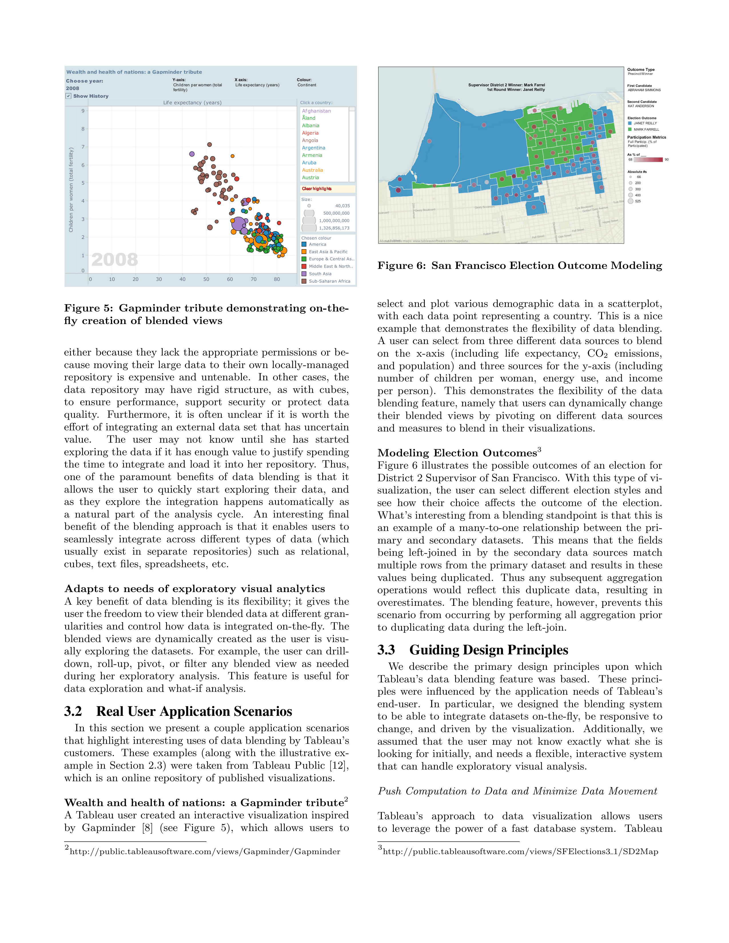
Figure
5:
Gapminder
tribute
demonstrating
on-the-
fly
creation
of
blended
views
either
because
they
lack
the
appropriate
permissions
or
be-
cause
moving
their
large
data
to
their
own
locally-managed
repository
is
expensive
and
untenable.
In
other
cases,
the
data
repository
may
have
rigid
structure,
as
with
cubes,
to
ensure
performance,
support
security
or
protect
data
quality.
Furthermore,
it
is
often
unclear
if
it
is
worth
the
effort
of
integrating
an
external
data
set
that
has
uncertain
value.
The
user
may
not
know
until
she
has
started
exploring
the
data
if
it
has
enough
value
to
justify
spending
the
time
to
integrate
and
load
it
into
her
repository.
Thus,
one
of
the
paramount
benefits
of
data
blending
is
that
it
allows
the
user
to
quickly
start
exploring
their
data,
and
as
they
explore
the
integration
happens
automatically
as
a
natural
part
of
the
analysis
cycle.
An
interesting
final
benefit
of
the
blending
approach
is
that
it
enables
users
to
seamlessly
integrate
across
different
types
of
data
(which
usually
exist
in
separate
repositories)
such
as
relational,
cubes,
text
files,
spreadsheets,
etc.
Adapts
to
needs
of
exploratory
visual
analytics
A
key
benefit
of
data
blending
is
its
flexibility;
it
gives
the
user the freedom to view their blended data at different gran-
ularities
and
control
how
data
is
integrated
on-the-fly.
The
blended
views
are
dynamically
created
as
the
user
is
visu-
ally
exploring
the
datasets.
For
example,
the
user
can
drill-
down,
roll-up,
pivot,
or
filter
any
blended
view
as
needed
during
her
exploratory
analysis.
This
feature
is
useful
for
data
exploration
and
what-if
analysis.
3.2
Real User Application Scenarios
In
this
section
we
present
a
couple
application
scenarios
that highlight interesting uses of data blending by Tableau’s
customers.
These
examples
(along
with
the
illustrative
ex-
ample
in
Section
2.3)
were
taken
from
Tableau
Public
[12],
which
is
an
online
repository
of
published
visualizations.
Wealth
and
health
of
nations:
a
Gapminder
tribute
2
A
Tableau
user
created
an
interactive
visualization
inspired
by
Gapminder
[8]
(see
Figure
5),
which
allows
users
to
2
http://public.tableausoftware.com/views/Gapminder/Gapminder
!"#$%&'()*+'
!"#$%&$'()%&&#"
!"#$%&'()*"*(%+
*+,*-*.(/0..12/
,+-.)*&'()*"*(%+
3*4(*256,/12
,-.#/$/+-#/%0(1'#./$2
7899(!:"'%$%;(?@(
!:"'%$%;:'#AB
!"#$%&'(")*($&+(,-.&///0%(")*($-#1%/(2*03#+4+(,5(%(
3"+'.4/2%.(5/2#./$#(6(7/00'.8(1-.9(:-..';
(7/00'.8(?-0'#(='/;;*
/0$.12%+&3$
CC
DEE
FEE
GEE
HDH
CI
JE
/$&4&.5&666
71+-%".)&82%-.9+
K*264(,60LLM
.*,3(7*,,6LL
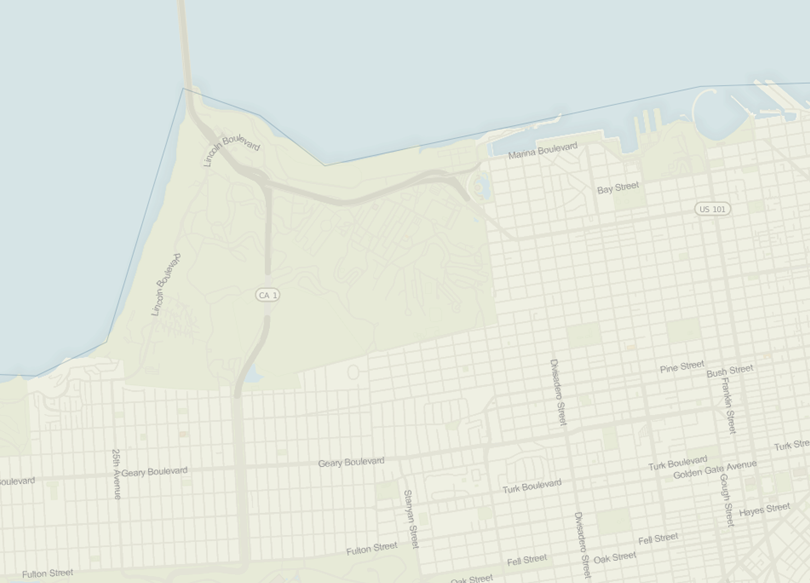
Figure
6:
San
Francisco
Election
Outcome
Modeling
select
and
plot
various
demographic
data
in
a
scatterplot,
with
each
data
point
representing
a
country.
This
is
a
nice
example
that
demonstrates
the
flexibility
of
data
blending.
A
user
can
select
from
three
different
data
sources
to
blend
on
the
x-axis
(including
life
expectancy,
CO
2
emissions,
and
population)
and
three
sources
for
the
y-axis
(including
number
of
children
per
woman,
energy
use,
and
income
per
person).
This
demonstrates
the
flexibility
of
the
data
blending feature,
namely that users can dynamically change
their
blended
views
by
pivoting
on
different
data
sources
and
measures
to
blend
in
their
visualizations.
Modeling
Election
Outcomes
3
Figure
6
illustrates
the
possible
outcomes
of
an
election
for
District 2 Supervisor of San Francisco.
With this type of vi-
sualization,
the
user
can
select
different
election
styles
and
see
how
their
choice
affects
the
outcome
of
the
election.
What’s interesting from a blending standpoint is that this is
an
example
of
a
many-to-one
relationship
between
the
pri-
mary
and
secondary
datasets.
This
means
that
the
fields
being
left-joined
in
by
the
secondary
data
sources
match
multiple
rows
from
the
primary
dataset
and
results
in
these
values
being
duplicated.
Thus
any
subsequent
aggregation
operations
would
reflect
this
duplicate
data,
resulting
in
overestimates.
The
blending
feature,
however,
prevents
this
scenario
from
occurring
by
performing
all
aggregation
prior
to
duplicating
data
during
the
left-join.
3.3
Guiding Design Principles
We
describe
the
primary
design
principles
upon
which
Tableau’s
data
blending
feature
was
based.
These
princi-
ples
were
influenced
by
the
application
needs
of
Tableau’s
end-user.
In
particular,
we
designed
the
blending
system
to
be
able
to
integrate
datasets
on-the-fly,
be
responsive
to
change,
and
driven
by
the
visualization.
Additionally,
we
assumed
that
the
user
may
not
know
exactly
what
she
is
looking
for
initially,
and
needs
a
flexible,
interactive
system
that
can
handle
exploratory
visual
analysis.
Push
Computation
to
Data
and
Minimize
Data
Movement
Tableau’s
approach
to
data
visualization
allows
users
to
leverage
the
power
of
a
fast
database
system.
Tableau
3
http://public.tableausoftware.com/views/SFElections3
1/SD2Map



































































compiles
the
VizQL
[10]
declarative
formalism
representing
a
visual
specification
into
SQL
or
MDX
and
pushes
this
computation
close
to
the
data,
where
the
fast
database
system
handles
computationally
intensive
aggregation
and
filtering
operations.
In
response,
the
database
provides
a
relatively
small
result
set
for
Tableau
to
render.
This
is
an
important
factor
in
Tableau’s
choice
of
post-aggregate
data
integration
across
disparate
data
sources
–
since
the
integrated
result
sets
must
represent
a
cognitively
manageable
amount
of
information,
the
data
integration
process
operates
on
small
amounts
of
aggregated,
fil-
tered
data
from
each
data
source.
This
approach
avoids
the
costly
migration
effort
to
collocate
massive
data
sets
in
a
single
warehouse,
and
continues
to
leverage
fast
databases for performing expensive queries close to the data.
Automate
as
Much
as
Possible,
but
Keep
User
in
Loop
Tableau’s
primary
focus
has
been
on
ease
of
use
since
most
of
Tableau’s
end-users
are
not
database
experts,
but
range
from
a
variety
of
domains
and
disciplines:
business
analysts,
journalists,
scientists,
students,
etc.
We
therefore,
took
a
simple,
pay-as-you-go
[3]
integration
approach
in
which
the
user
invests
minimal
upfront
effort
or
time
to
receive
the
benefits
of
the
system.
For
example,
the
data
blending
system
does
not
require
the
user
to
specify
schemas
for
their
data
sets,
rather
the
system
tries
to
infer
this
information
as
well
as
how
to
apply
schema
matching
techniques
to
blend
them
for
a
given
visualization.
Further-
more
the
system
provides
a
simple
drag-and-drop
interface
for
the
user
to
specify
the
fields
for
a
visualization,
and
if
there
are
fields
from
multiple
data
sources
in
play
at
the
same
time,
the
blending
system
infers
how
to
join
them
to
satisfy
the
needs
of
the
visualization.
In
the
case
that
something
goes
wrong,
for
example,
if
the
schema
matching
could
not
succeed,
the
blending
sys-
tem
provides
a
simple
interface
for
specifying
data
source
relationships
and
how
blending
should
proceed.
Addition-
ally,
the
system
provides
several
techniques
for
managing
the
impact
of
dirty
data
on
blending,
which
we
discuss
in
Section
4.8
4.
INTEGRATING DATA IN TABLEAU
In this section we discuss in greater detail how data blend-
ing
works.
Then
we
discuss
how
a
user
builds
visualizations
using
data
blending
using
several
large
datasets
involving
airline
statistics.
4.1
Data Blending Architecture
The
data
blending
system,
shown
in
Figure
7
takes
as
in-
put
the
VizQL
query
workload
generated
by
the
user’s
GUI
actions
and
data
source
schemas,
and
automatically
infers
how
to
query
the
data
sources
remotely
and
combine
their
results
on-the-fly.
The
system
features
a
two-tier
mediator-
based architecture in which the VizQL query workload is an-
alyzed
and
partitioned
at
runtime
based
on
the
correspond-
ing data source fields being used.
The primary mediator ini-
tiates this process by removing the visual encodings from the
VizQL
query
workload
to
yield
an
abstract
query
.
The
ab-
stract
query
is
partitioned
for
further
processing
by
the
pri-
mary
mediator
and
one
or
more
secondary
mediators.
The
primary mediator creates the mediated schema for the given
query workload.
It then federates the abstract queries to the
Data Marts
Data
Warehouse
Files
Cubes
Primary data source
!
Secondary data source(s)
!
"#$#!$%!&'()'*'*+!
,-+$*#.$!/0'*1!
234!5!6"7!/0'*1!
30'*1!8%*9:%#)!;34?!
&'+0:$!+'$!
Data Marts
Data
Warehouse
Files
@*=A#*1!,)#BCD'!6')=#$%*!
@#*CC%(!E%*9:%#)!
Result set
Wrapper
Wrapper
Wrapper
Wrappers
2'.%()#*1!6')=#$%*+!
F#-:'#0!
Figure
7:
Tableau’s
Data
Blending
Architecture
primary
data
source
as
well
as
the
secondary
mediators
and
their
respective
data
sources.
The
wrappers
compile
the
abstract
queries
into
concrete
SQL
or
MDX
queries
and
in-
stantiate
the
semantic
mappings
between
the
data
sources
and
the
mediated
schema
for
each
query.
The
primary
me-
diator
joins
all
the result sets returned from all
data
sources
to
produce
the
mediated
result
set
used
by
the
rendering
system.
c
d
!"#$%"&'(%)%'*+,"-.'
/.-+0(%"&'
(%)%'*+,"-.*'
b
a
b
c
d
a
!"#$%&"#'()*"+%'
,'
-.$+%./'0"/'1$"2#('
34$5'0"/('
Figure
8:
Components
of
the
Mediated
Schema
4.2
Post-aggregate Join
A
visualization
is
organized
by
its
discrete
fields
into
pages,
partitions,
colors,
etc.,
and
like
a
GROUP
BY
clause
in
SQL,
these
grouping
fields
comprise
the
primary
key
of
the
visualization.
In
a
blended
visualization,
the
grouping
fields from the primary data source become the primary key
of
the
mediated
schema.
In
Figure
8
these
are
shown
as
the
dark-green
fields
in
the
primary
data
source,
and
the
light-
green
fields
represent
the
aggregated
data.
Each
secondary
data
source
must
contain
at
least
one
field
that
matches
a
visualization
grouping
field
in
order
to
blend
into
the
me-
diated
schema.
The
matching
fields
in
a
secondary
data
source comprise its join key, and fields appear in the GROUP
BY
clause
issued
by
the
secondary
mediator
wrappers.
The
aggregated
data
from
the
secondary
data
source,
shown
in
light-purple,
is
then
left-joined
along
its
join
key
into
the
mediated
result
set.
We
refer
to
this
left-join
of
aggregated
result
sets
as
a
post-aggregate
join
.
(a)
(b)
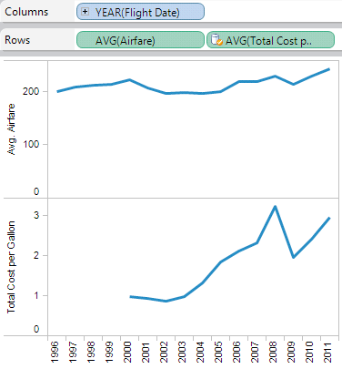
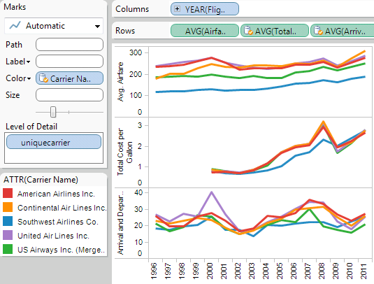
Figure
9:
Screenshots
of
Blended
Airline
Data
from
Bureau
of
Transportation
Statistics:
(a)
Airfare
Price
(324M
rows)
and
Fuel
Costs
(8K
rows)
by
year
(b)
Both
datasets
from
(a),
On-Time
Performance
(140M
rows),
and
Carrier
Names
(1.5K
rows).
4.3
Primary Key Cardinality
As
a
user
blends
additional
data
into
her
visualization,
she
is
guaranteed
that
the
blended
data
will
not
affect
the
cardinality
of
the
result
set.
The
left-join
ensures
that
no
rows
from
the
primary
data
source
result
set
are
lost
due
to
missing
data
from
a
secondary
data
source.
Additionally
there cannot be a one-to-many mapping between the domain
values of the primary key and those of the secondary join key,
because the secondary join key is a subset of the primary key
and contains only unique values in the aggregated secondary
result
set.
We
find
that
this
approach
is
the
most
natural
for
augmenting
a
visualization
with
secondary
data
sources
of
uncertain
value
or
quality,
which
is
a
common
scenario
for
Tableau
users.
Data
blending
supports
many-to-one
relationships
be-
tween the primary and each secondary.
This can occur when
the
secondary
data
source
contains
coarser-grained
data
than
the
mediated
result
set,
as
discussed
in
Section
3.1.
Since
the
join
key
in
a
secondary
result
set
may
match
a
subset
of
the
blended
result
set
primary
key,
portions
of
the
secondary
result
set
may
be
duplicated
across
repeated
val-
ues
in
the
mediated
result
set.
This
does
not
pose
risk
of
double-counting
measure
values,
becaused
all
aggregation
is
performed
prior
to
the
join.
When
a
blended
visualization
uses
multiple
secondary
data
sources,
each
secondary
join
key
may
match
any
subset
of
the
primary
key.
The
primary
mediator
handles
duplicating
each
secondary
result
set
as
needed
to
join
with
the
mediated
result
set.
Finally,
a
secondary
dimension
which
is
not
part
of
the
join
key
(and
thus
not
a
grouping
field
in
the
secondary
query) can still be used in the visualization.
If it is function-
ally dependent on the join key, a secondary dimension can be
used without affecting the result set cardinality.
Tableau ref-
erences this kind of non-grouping dimension using both MIN
and MAX aggregations in the query issued to the secondary
data
source,
which
allows
Tableau
to
determine
if
the
di-
mension
is
functionally
dependent
on
the
join
key.
For
each
row
in
the
secondary
result
set,
if
the
two
aggregated
values
are the same then the value is used as-is, reflecting the func-
tional
dependence
on
the
grouping
fields.
If
the
aggregated
values
differ,
Tableau
represents
the
value
using
a
special
form
of
NULL
called
ManyValues
.
This
is
represented
in
the
visualization
as
a
‘*’,
but
retains
the
behavior
of
NULL
when
used
in
calculated
fields
or
other
computations.
The
visual
feedback
allows
a
user
to
distinguish
this
lack
of
data
from
the
NULLs
which
occur
due
to
missing
or
mismatched
data.
4.4
Inferring Join Keys
Tableau
uses
very
simple
rules
for
automatically
detect-
ing
candidate
join
keys:
1)
the
secondary
data
source
field
name
must
match
a
field
with
the
same
name
in
the
pri-
mary
data
source,
2)
the
data
types
must
match
3)
if
they
are
date/time
fields,
they
must
represent
the
same
granu-
larity
date
bin
in
the
date/time
hierarchy,
e.g.
both
are
MONTH.
A
user
can
intervene
to
force
a
match
either
by
providing
field
captions
to
rename
fields
within
the
Tableau
data
model,
or
by
explicitly
defining
a
link
between
fields
using
a
simple
user
interface.
4.5
Simple Blending Example
A
Tableau
data
blending
scenario
is
shown
in
Figure
9,
which
includes
multiple
views
that
were
composed
in
min-
utes
by
uniquely
mashing
up
four
different
airline
datasets,
the
largest
of
which
include
a
324
million
row
ticket
pric-
ing
database
and
a
140
million
row
on-time
performance
database.
A
user
starts
by
dragging
fields
from
any
dataset
on
to
a
blank
visual
canvas,
iteratively
building
a
VizQL
statement which ultimately produces a visualization.
In this
example,
the
user
first
drags
the
VizQL
fields,
YEAR(Flight
Date)
and
AVG(Airfare)
,
from
the
pricing
dataset
onto
the
visual
canvas.
Data
blending
occurs
when
the
user
adds
fields
from
a
separate
dataset
to
an
existing
VizQL
statement
in
order
to
augment
their
analysis.
Tableau
assigns
the
existing
dataset
to
the
primary
mediator
and
uses
secondary
me-
diators
to
manage
each
subsequent
dataset
added
to
the
VizQL.
The
mediated
schema
has
a
primary
key
composed
of
the
grouping
VizQL
fields
from
the
primary
dataset
(
e.g.
YEAR(Flight
Date)
);
the
remaining
fields
in
the
mediated
schema
are
the
aggregated
VizQL
fields
from
the
primary
dataset
along
with
the
VizQL
fields
from
each
secondary
dataset.
Continuing
our
example,
the
user
wishes
to
drag
AVG(Total
Cost
per
Gallon)
from
the
fuel
cost
dataset
to
the visualization.
The schema matching algorithm examines
the secondary dataset for one or more fields whose name ex-
actly
matches
a
field
in
the
primary
key
of
the
mediated
schema.
While
the
proposed
matches
are
often
sufficient
and
acceptable,
the
user
can
specify
an
override.
Since
the
fuel cost dataset has a field named
Date
,
the user provides a
caption
of
Flight
Date
to
resolve
the
schema
discrepancy.
At
this
point
the
mediated
schema
is
created
and
the
VizQL
workload
is
then
federated
to
the
wrappers
for
each
dataset.
Each
wrapper
compiles
VizQL
to
SQL
or
MDX
for
the
given
workload,
executes
the
query,
and
maps
the
result
set
into
the
intermediate
form
expected
by
the
primary
me-
diator.
The
mapping
is
performed
dynamically,
since
both
the
VizQL
and
the
data
model
evolve
during
a
user’s
it-
erative
analytical
workflow.
Finally,
the
primary
mediator
performs
a
left-join
of
each
secondary
result
set
along
the
primary
key
of
the
mediated
schema.
In
this
example,
the
mediated
result
set
is
rendered
to
produce
the
visualization
shown
in
Figure
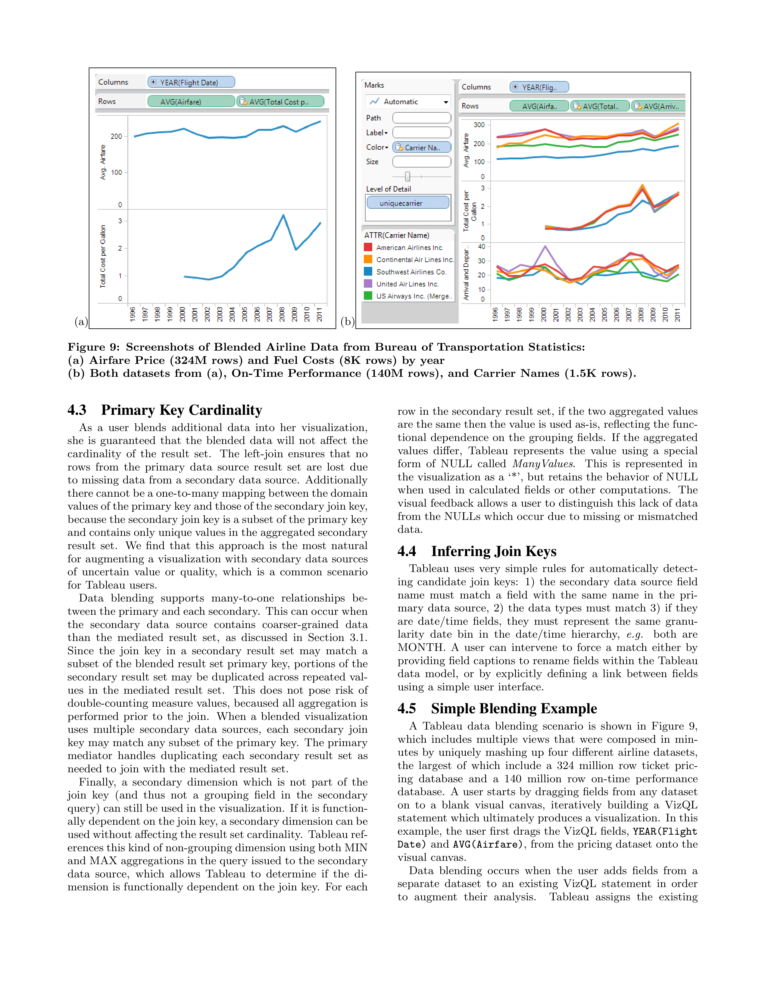
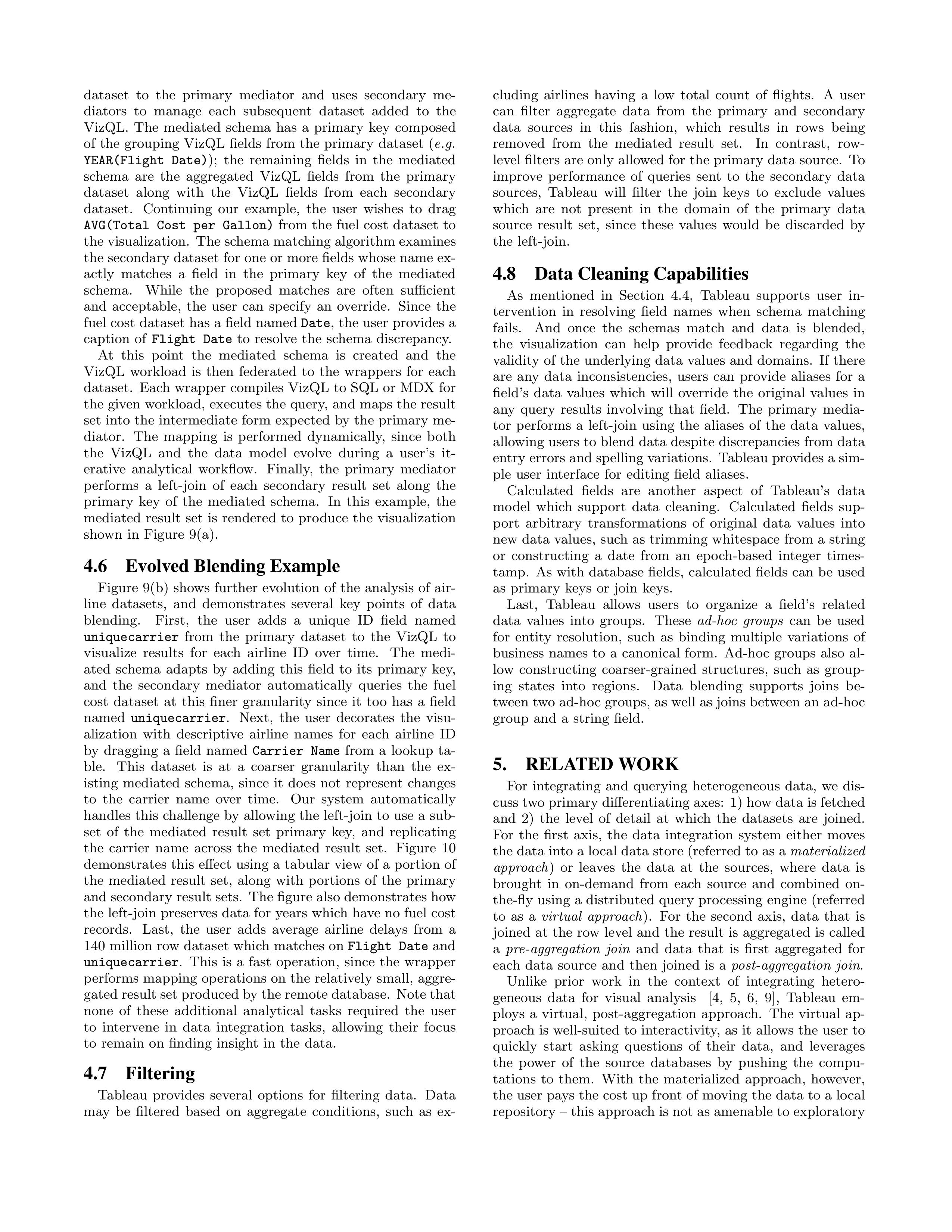
9(a).
4.6
Evolved Blending Example
Figure
9(b)
shows
further
evolution
of
the
analysis
of
air-
line
datasets,
and
demonstrates
several
key
points
of
data
blending.
First,
the
user
adds
a
unique
ID
field
named
uniquecarrier
from
the
primary
dataset
to
the
VizQL
to
visualize
results
for
each
airline
ID
over
time.
The
medi-
ated
schema
adapts
by
adding
this
field
to
its
primary
key,
and
the
secondary
mediator
automatically
queries
the
fuel
cost
dataset
at
this
finer
granularity
since
it
too
has
a
field
named
uniquecarrier
.
Next,
the
user
decorates
the
visu-
alization
with
descriptive
airline
names
for
each
airline
ID
by
dragging
a
field
named
Carrier
Name
from
a
lookup
ta-
ble.
This
dataset
is
at
a
coarser
granularity
than
the
ex-
isting
mediated
schema,
since
it
does
not
represent
changes
to
the
carrier
name
over
time.
Our
system
automatically
handles
this
challenge
by
allowing
the
left-join
to
use
a
sub-
set
of
the
mediated
result
set
primary
key,
and
replicating
the
carrier
name
across
the
mediated
result
set.
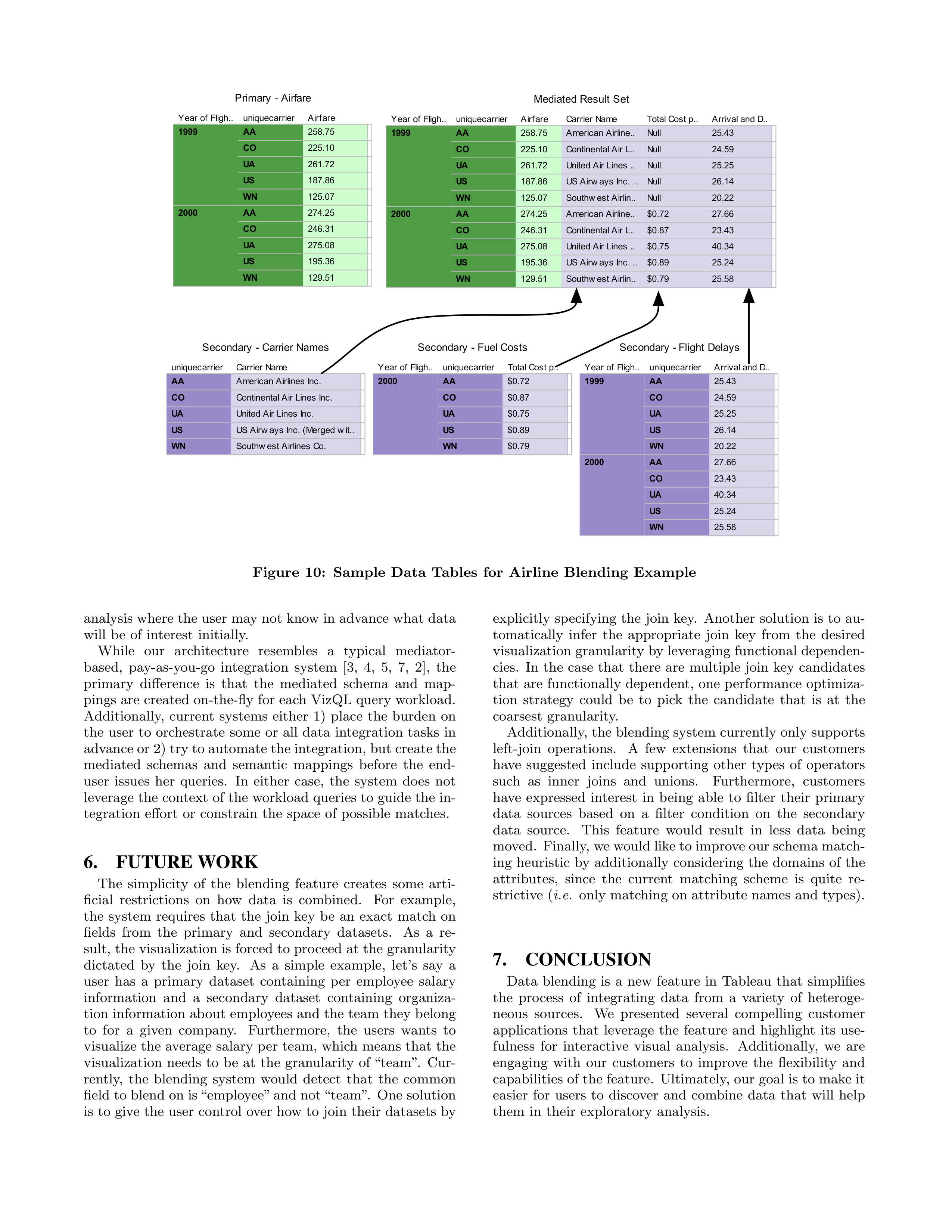
Figure
10
demonstrates
this
effect
using
a
tabular
view
of
a
portion
of
the
mediated
result
set,
along
with
portions
of
the
primary
and secondary result sets.
The figure also demonstrates how
the
left-join
preserves
data
for
years
which
have
no
fuel
cost
records.
Last,
the
user
adds
average
airline
delays
from
a
140
million
row
dataset
which
matches
on
Flight
Date
and
uniquecarrier
.
This
is
a
fast
operation,
since
the
wrapper
performs
mapping
operations
on
the
relatively
small,
aggre-
gated result set produced by the remote database.
Note that
none
of
these
additional
analytical
tasks
required
the
user
to
intervene
in
data
integration
tasks,
allowing
their
focus
to
remain
on
finding
insight
in
the
data.
4.7
Filtering
Tableau
provides
several
options
for
filtering
data.
Data
may
be
filtered
based
on
aggregate
conditions,
such
as
ex-
cluding
airlines
having
a
low
total
count
of
flights.
A
user
can
filter
aggregate
data
from
the
primary
and
secondary
data
sources
in
this
fashion,
which
results
in
rows
being
removed
from
the
mediated
result
set.
In
contrast,
row-
level filters are only allowed for the primary data source.
To
improve
performance
of
queries
sent
to
the
secondary
data
sources,
Tableau
will
filter
the
join
keys
to
exclude
values
which
are
not
present
in
the
domain
of
the
primary
data
source
result
set,
since
these
values
would
be
discarded
by
the
left-join.
4.8
Data Cleaning Capabilities
As
mentioned
in
Section
4.4,
Tableau
supports
user
in-
tervention
in
resolving
field
names
when
schema
matching
fails.
And
once
the
schemas
match
and
data
is
blended,
the
visualization
can
help
provide
feedback
regarding
the
validity
of
the
underlying
data
values
and
domains.
If
there
are
any
data
inconsistencies,
users
can
provide
aliases
for
a
field’s
data
values
which
will
override
the
original
values
in
any
query
results
involving
that
field.
The
primary
media-
tor
performs
a
left-join
using
the
aliases
of
the
data
values,
allowing users to blend data despite discrepancies from data
entry errors and spelling variations.
Tableau provides a sim-
ple
user
interface
for
editing
field
aliases.
Calculated
fields
are
another
aspect
of
Tableau’s
data
model
which
support
data
cleaning.
Calculated
fields
sup-
port
arbitrary
transformations
of
original
data
values
into
new
data
values,
such
as
trimming
whitespace
from
a
string
or
constructing
a
date
from
an
epoch-based
integer
times-
tamp.
As
with
database
fields,
calculated
fields
can
be
used
as
primary
keys
or
join
keys.
Last,
Tableau
allows
users
to
organize
a
field’s
related
data
values
into
groups.
These
ad-hoc
groups
can
be
used
for
entity
resolution,
such
as
binding
multiple
variations
of
business
names
to
a
canonical
form.
Ad-hoc
groups
also
al-
low
constructing
coarser-grained
structures,
such
as
group-
ing
states
into
regions.
Data
blending
supports
joins
be-
tween two ad-hoc groups, as well as joins between an ad-hoc
group
and
a
string
field.
5.
RELATED WORK
For
integrating
and
querying
heterogeneous
data,
we
dis-
cuss two primary differentiating axes:
1) how data is fetched
and
2)
the
level
of
detail
at
which
the
datasets
are
joined.
For
the
first
axis,
the
data
integration
system
either
moves
the data into a local data store (referred to as a
materialized
approach
)
or
leaves
the
data
at
the
sources,
where
data
is
brought
in
on-demand
from
each
source
and
combined
on-
the-fly
using
a
distributed
query
processing
engine
(referred
to
as
a
virtual
approach
).
For
the
second
axis,
data
that
is
joined
at
the
row
level
and
the
result
is
aggregated
is
called
a
pre-aggregation
join
and
data
that
is
first
aggregated
for
each
data
source
and
then
joined
is
a
post-aggregation
join
.
Unlike
prior
work
in
the
context
of
integrating
hetero-
geneous
data
for
visual
analysis
[4,
5,
6,
9],
Tableau
em-
ploys
a
virtual,
post-aggregation
approach.
The
virtual
ap-
proach
is
well-suited
to
interactivity,
as
it
allows
the
user
to
quickly
start
asking
questions
of
their
data,
and
leverages
the
power
of
the
source
databases
by
pushing
the
compu-
tations
to
them.
With
the
materialized
approach,
however,
the user pays the cost up front of moving the data to a local
repository – this approach is not as amenable to exploratory
!"#$%&'%()*+,--
./*0."1#$$*"$
2*$'#$"
3#$$*"$%4#5"
6&7#)%3&87%9--
2$$*:#)%#/;%<--
!"""
##
=>?-@>
25"$*1#/%2*$)*/"--
4.))
=>-AB
$%
==>-CD
3&/7*/"/7#)%2*$%E--
4.))
=A->F
&#
=GC-@=
H/*7";%2*$%E*/"8%--
4.))
=>-=>
&'
C?@-?G
HI%2*$J #K8%L/1-%--
4.))
=G-CA
()
C=>-D@
I&.7,J "87%2*$)*/--
4.))
=D-==
*+++
##
=@A-=>
25"$*1#/%2*$)*/"--
MD-@=
=@-GG
$%
=AG-BC
3&/7*/"/7#)%2*$%E--
MD-?@
=B-AB
&#
=@>-D?
H/*7";%2*$%E*/"8%--
MD-@>
AD-BA
&'
CF>-BG
HI%2*$J #K8%L/1-%--
MD-?F
=>-=A
()
C=F->C
I&.7,J "87%2*$)*/--
MD-@F
=>->?
!"#$%&"#'(")*+&',"&
!"#$%&'%()*+,--
./*0."1#$$*"$
2*$'#$"
!"""
##
345-64
$%
334-78
&#
397-63
&'
756-59
()
734-86
*+++
##
36:-34
$%
3:9-;7
&#
364-85
&'
7<4-;9
()
73<-47
!"#$%"&'(')#"*%"+
!"#$!%&'((#%(
)'((#%(*+',%
!!
-,%(#&'"*-#(.#"%/*0"&1
"#
)2"3#"%"3'.*-#(*4#"%/*0"&1
$!
5"#3%6*-#(*4#"%/*0"&1
$%
57*-#(8 '9/*0"&1*:;%(<%6*8 #311
&'
72!3=8 %/3*-#(.#"%/*)21
!"#$%&'()*+*,'((-"(*.'/"0
>%'(*2?*@.#<=11
!"#$!%&'((#%(
-((#A'.*'"6*B11
()))
!!
CD1EF
"#
CE1DG
$!
CD1CD
$%
CH1IE
&'
CJ1CC
*+++
!!
CK1HH
"#
CF1EF
$!
EJ1FE
$%
CD1CE
&'
CD1DL
!"#$%&'()*+*12-345*6"2')0
>%'(*2?*@.#<=11
!"#$!%&'((#%(
M23'.*)2/3*N11
*+++
!!
OJ1KC
"#
OJ1LK
$!
OJ1KD
$%
OJ1LG
&'
OJ1KG
!"#$%&'()*+*17"2*,$050
Figure
10:
Sample
Data
Tables
for
Airline
Blending
Example
analysis where the user may not know in advance what data
will
be
of
interest
initially.
While
our
architecture
resembles
a
typical
mediator-
based,
pay-as-you-go
integration
system
[3,
4,
5,
7,
2],
the
primary
difference
is
that
the
mediated
schema
and
map-
pings are created on-the-fly for each VizQL query workload.
Additionally,
current
systems
either
1)
place
the
burden
on
the
user
to
orchestrate
some
or
all
data
integration
tasks
in
advance or 2) try to automate the integration, but create the
mediated
schemas
and
semantic
mappings
before
the
end-
user
issues
her
queries.
In
either
case,
the
system
does
not
leverage the context of the workload queries to guide the in-
tegration
effort
or
constrain
the
space
of
possible
matches.
6.
FUTURE WORK
The
simplicity
of
the
blending
feature
creates
some
arti-
ficial
restrictions
on
how
data
is
combined.
For
example,
the
system
requires
that
the
join
key
be
an
exact
match
on
fields
from
the
primary
and
secondary
datasets.
As
a
re-
sult,
the visualization is forced to proceed at the granularity
dictated
by
the
join
key.
As
a
simple
example,
let’s
say
a
user
has
a
primary
dataset
containing
per
employee
salary
information
and
a
secondary
dataset
containing
organiza-
tion information about employees and the team
they belong
to
for
a
given
company.
Furthermore,
the
users
wants
to
visualize
the
average
salary
per
team,
which
means
that
the
visualization
needs
to
be
at
the
granularity
of “team”.
Cur-
rently,
the
blending
system
would
detect
that
the
common
field to blend on is “employee” and not “team”.
One solution
is
to
give
the
user
control
over
how
to
join
their
datasets
by
explicitly
specifying
the
join
key.
Another
solution
is
to
au-
tomatically
infer
the
appropriate
join
key
from
the
desired
visualization granularity by leveraging functional dependen-
cies.
In
the
case
that
there
are
multiple
join
key
candidates
that
are
functionally
dependent,
one
performance
optimiza-
tion
strategy
could
be
to
pick
the
candidate
that
is
at
the
coarsest
granularity.
Additionally, the blending system currently only supports
left-join
operations.
A
few
extensions
that
our
customers
have
suggested
include
supporting
other
types
of
operators
such
as
inner
joins
and
unions.
Furthermore,
customers
have
expressed
interest
in
being
able
to
filter
their
primary
data
sources
based
on
a
filter
condition
on
the
secondary
data
source.
This
feature
would
result
in
less
data
being
moved.
Finally, we would like to improve our schema match-
ing
heuristic
by
additionally
considering
the
domains
of
the
attributes,
since
the
current
matching
scheme
is
quite
re-
strictive
(
i.e.
only
matching
on
attribute
names
and
types).
7.
CONCLUSION
Data
blending
is
a
new
feature
in
Tableau
that
simplifies
the
process
of
integrating
data
from
a
variety
of
heteroge-
neous
sources.
We
presented
several
compelling
customer
applications
that
leverage
the
feature
and
highlight
its
use-
fulness
for
interactive
visual
analysis.
Additionally,
we
are
engaging
with
our
customers
to
improve
the
flexibility
and
capabilities of the feature.
Ultimately, our goal is to make it
easier
for
users
to
discover
and
combine
data
that
will
help
them
in
their
exploratory
analysis.
8.
ACKNOWLEDGEMENTS
We
thank
Magdalena
Balazinska,
AnHai
Doan,
Dan
Grossman,
Alon
Halevy,
and
Richard
Wesley
for
their
help-
ful
feedback
on
earlier
versions
of
this
paper.
9.
REFERENCES
[1]
S.K.
Card,J.
Mackinlay,B.
Shneiderman.
Readings
in
Information
Visualization:
Using
Vision
To
Think
.
Morgan-Kaufmann:
San
Francisco,
CA,
1999.
[2]
A.
Das
Sarma,
X.
Dong,
and
A.
Halevy.
Bootstrapping
Pay-As-You-Go
Data
Integration
Systems
In
SIGMOD
,
2008.
[3]
M.
Franklin,
A.
Halevy,
and
D.
Maier.
From
databases
to
dataspaces:
a
new
abstraction
for
information
management.
In
SIGMOD
Rec.
,
2005.
[4]
H.
Gonzalez,
A.
Halevy,
C.
Jensen,
A.
Langen,
J.
Madhavan,
R.
Shapley,
and
W.
Shen.
Google
Fusion
Tables:
Data
Management,
Integration
and
Collaboration
in
the
Cloud.
In
SoCC
,
2010.
[5]
H.
Gonzalez,
A.
Halevy,
C.
Jensen,
A.
Langen,
J.
Madhavan,
R.
Shapley,
W.
Shen,
and
J.
Goldberg-Kidon.
Google
Fusion
Tables:
Web-Centered
Data
Management
and
Collaboration.
In
SIGMOD
Conference
,
2010.
[6]
QlikView,
2012.
http://www.qlikview.com
.
[7]
M.
Hentschel,
L.
Haas,
R.
Miller.
Just-in-time
Data
Integration
in
Action
In
VLDB
,
2010.
[8]
H.
Rosling.
GapMinder
Foundation,
2012.
http://www.gapminder.org/
[9]
Spotfire,
2012.
http://spotfire.tibco.com
.
[10]
C.
Stolte,
D.
Tang,
and
P.
Hanrahan.
Polaris:
a
system
for
query,
analysis,
and
visualization
of
multidimensional
databases.
In
IEEE
Transaction
on
Visualization
and
Computer
Graphics
,
2002.
[11]
Tableau
Software,
2012.
http://www.tableausoftware.com
.
[12]
Tableau
Software,
2012.
http://www.tableaupublic.com
.
[13]
F.
B.
Viegas,
M.
Wattenberg,
F.
van
Ham,
J.
Kriss,
M.
McKeon.
Many
Eyes:
A
Site
for
Visualization
at
Internet
Scale.
In
IEEE
Transactions
on
Visualization
and
Computer
Graphics
,
vol.
13,
no.
6,
pp.
1121-1128,
Nov/Dec,
2007.