
Learning Transferable Visual Models From Natural Language Supervision
Alec Radford
* 1
Jong Wook Kim
* 1
Chris Hallacy
1
Aditya Ramesh
1
Gabriel Goh
1
Sandhini Agarwal
1
Girish Sastry
1
Amanda Askell
1
Pamela Mishkin
1
Jack Clark
1
Gretchen Krueger
1
Ilya Sutskever
1
Abstract
State-of-the-art
computer
vision
systems
are
trained
to
predict
a
fixed
set
of
predetermined
object categories.
This restricted form of super-
vision limits their generality and usability since
additional labeled data is needed to specify any
other visual concept.
Learning directly from raw
text about images is a promising alternative which
leverages a much broader source of supervision.
We demonstrate that the simple pre-training task
of predicting which caption goes with which im-
age is an efficient and scalable way to learn SOTA
image representations from scratch on a dataset
of 400 million (image, text) pairs collected from
the internet.
After pre-training, natural language
is
used
to
reference
learned
visual
concepts
(or
describe
new
ones)
enabling
zero-shot
transfer
of
the
model
to
downstream
tasks.
We
study
the performance of this approach by benchmark-
ing
on
over
30
different
existing
computer
vi-
sion
datasets,
spanning
tasks
such
as
OCR,
ac-
tion recognition in videos, geo-localization, and
many types of fine-grained object classification.
The
model
transfers
non-trivially
to
most
tasks
and is often competitive with a fully supervised
baseline
without
the
need
for
any
dataset
spe-
cific
training.
For
instance,
we
match
the
ac-
curacy
of
the
original
ResNet-50
on
ImageNet
zero-shot without needing to use any of the 1.28
million training examples it was trained on.
We
release our code and pre-trained model weights at
https://github.com/OpenAI/CLIP
.
1. Introduction and Motivating Work
Pre-training
methods
which
learn
directly
from
raw
text
have
revolutionized
NLP
over
the
last
few
years
(
Dai
&
Le
,
2015
;
Peters et al.
,
2018
;
Howard & Ruder
,
2018
;
Rad-
ford
et
al.
,
2018
;
Devlin
et
al.
,
2018
;
Raffel
et
al.
,
2019
).
*
Equal contribution
1
OpenAI, San Francisco, CA 94110, USA.
Correspondence to:
<
{
alec, jongwook
}
@openai.com
>
.
Task-agnostic objectives such as autoregressive and masked
language modeling have scaled across many orders of mag-
nitude in compute,
model capacity,
and data,
steadily im-
proving capabilities.
The development of “text-to-text” as
a standardized input-output interface (
McCann et al.
,
2018
;
Radford et al.
,
2019
;
Raffel et al.
,
2019
) has enabled task-
agnostic architectures to zero-shot transfer to downstream
datasets removing the need for specialized output heads or
dataset specific customization.
Flagship systems like GPT-3
(
Brown et al.
,
2020
) are now competitive across many tasks
with
bespoke
models
while
requiring
little
to
no
dataset
specific training data.
These results suggest that the aggregate supervision acces-
sible to modern pre-training methods within web-scale col-
lections of text surpasses that of high-quality crowd-labeled
NLP datasets.
However,
in other fields such as computer
vision
it
is
still
standard
practice
to
pre-train
models
on
crowd-labeled datasets such as ImageNet (
Deng et al.
,
2009
).
Could
scalable
pre-training
methods
which
learn
directly
from web text result in a similar breakthrough in computer
vision?
Prior work is encouraging.
Over 20 years ago
Mori et al.
(
1999
) explored improving
content
based
image
retrieval
by
training
a
model
to
pre-
dict the nouns and adjectives in text documents paired with
images.
Quattoni et al.
(
2007
) demonstrated it was possi-
ble to learn more data efficient image representations via
manifold learning in the weight space of classifiers trained
to
predict
words
in
captions
associated
with
images.
Sri-
vastava
&
Salakhutdinov
(
2012
)
explored
deep
represen-
tation
learning
by
training
multimodal
Deep
Boltzmann
Machines on top of low-level image and text tag features.
Joulin et al.
(
2016
) modernized this line of work and demon-
strated
that
CNNs
trained
to
predict
words
in
image
cap-
tions
learn
useful
image
representations.
They
converted
the title, description, and hashtag metadata of images in the
YFCC100M
dataset
(
Thomee
et
al.
,
2016
)
into
a
bag-of-
words multi-label classification task and showed that pre-
training AlexNet (
Krizhevsky et al.
,
2012
) to predict these
labels
learned
representations
which
preformed
similarly
to ImageNet-based pre-training on transfer tasks.
Li et al.
(
2017
) then extended this approach to predicting phrase n-
grams in addition to individual words and demonstrated the
ability of their system to zero-shot transfer to other image
arXiv:2103.00020v1 [cs.CV] 26 Feb 2021

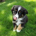
Learning Transferable Visual Models From Natural Language Supervision
2
I
1
·T
2
I
1
·T
3
…
I
2
·T
1
I
2
·T
3
…
I
3
·T
1
I
3
·T
2
…
⋮
⋮
⋮
I
1
·T
1
I
2
·T
2
I
3
·T
3
(1) Contrastive pre-training
Image
Encoder
Text
Encoder
Pepper the
aussie pup
Pepper the
aussie pup
Pepper the
aussie pup
Pepper the
aussie pup
T
1
T
2
T
3
…
I
1
I
2
I
3
⋮
(2) Create dataset classifier from label text
plane
car
dog
⋮
bird
A photo of
a
{object}
.
⋮
Text
Encoder
T
1
T
2
T
3
T
N
…
(3) Use for zero-shot prediction
Image
Encoder
I
1
I
1
·T
2
I
1
·T
N
I
1
·T
1
…
…
A photo of
a
dog
.
T
N
I
N
·T
1
I
N
·T
2
I
N
·T
3
I
1
·T
N
I
2
·T
N
I
3
·T
N
⋮
…
I
N
…
⋮
⋱
I
N
·T
N
I
1
·T
3
Figure 1.
Summary of our approach.
While standard image models jointly train an image feature extractor and a linear classifier to predict
some label, CLIP jointly trains an image encoder and a text encoder to predict the correct pairings of a batch of (image, text) training
examples.
At test time the learned text encoder synthesizes a zero-shot linear classifier by embedding the names or descriptions of the
target dataset’s classes.
classification
datasets
by
scoring
target
classes
based
on
their dictionary of learned visual n-grams and predicting the
one with the highest score.
Adopting more recent architec-
tures and pre-training approaches, VirTex (
Desai & Johnson
,
2020
),
ICMLM (
Bulent Sariyildiz et al.
,
2020
),
and Con-
VIRT (
Zhang et al.
,
2020
) have recently demonstrated the
potential of transformer-based language modeling, masked
language modeling, and contrastive objectives to learn im-
age representations from text.
While exciting as proofs of concept, using natural language
supervision for image representation learning is still rare.
This is likely because demonstrated performance on com-
mon benchmarks is much lower than alternative approaches.
For
example,
Li
et
al.
(
2017
)
reach
only
11.5%
accuracy
on ImageNet in a zero-shot setting.
This is well below the
88.4%
accuracy
of
the
current
state
of
the
art
(
Xie
et
al.
,
2020
).
It is even below the 50% accuracy of classic com-
puter vision approaches (
Deng et al.
,
2012
).
Instead, more
narrowly scoped but well-targeted uses of weak supervision
have improved performance.
Mahajan et al.
(
2018
) showed
that predicting ImageNet-related hashtags on Instagram im-
ages is an effective pre-training task.
When fine-tuned to
ImageNet these pre-trained models increased accuracy by
over 5% and improved the overall state of the art at the time.
Kolesnikov et al.
(
2019
) and
Dosovitskiy et al.
(
2020
) have
also demonstrated large gains on a broader set of transfer
benchmarks by pre-training models to predict the classes of
the noisily labeled JFT-300M dataset.
This line of work represents the current pragmatic middle
ground between learning from a limited amount of super-
vised “gold-labels” and learning from practically unlimited
amounts
of
raw
text.
However,
it
is
not
without
compro-
mises.
Both works carefully design, and in the process limit,
their
supervision
to
1000
and
18291
classes
respectively.
Natural language is able to express, and therefore supervise,
a
much
wider
set
of
visual
concepts
through
its
general-
ity.
Both approaches also use static softmax classifiers to
perform prediction and lack a mechanism for dynamic out-
puts.
This severely curtails their flexibility and limits their
“zero-shot” capabilities.
A crucial difference between these weakly supervised mod-
els and recent explorations of learning image representations
directly from natural language is scale.
While
Mahajan et al.
(
2018
) and
Kolesnikov et al.
(
2019
) trained their models for
accelerator years on millions to billions of images, VirTex,
ICMLM, and ConVIRT trained for accelerator days on one
to
two
hundred
thousand
images.
In
this
work,
we
close
this gap and study the behaviors of image classifiers trained
with natural language supervision at large scale.
Enabled
by the large amounts of publicly available data of this form
on the internet, we create a new dataset of 400 million (im-
age, text) pairs and demonstrate that a simplified version of
ConVIRT trained from scratch, which we call CLIP, for Con-
trastive Language-Image Pre-training, is an efficient method
of
learning
from
natural
language
supervision.
We
study
the scalability of CLIP by training a series of eight models
spanning almost 2 orders of magnitude of compute and ob-
serve that transfer performance is a smoothly predictable
function of compute (
Hestness et al.
,
2017
;
Kaplan et al.
,
2020
).
We find that CLIP, similar to the GPT family, learns
to perform a wide set of tasks during pre-training including
OCR, geo-localization, action recognition, and many others.
We
measure
this
by
benchmarking
the
zero-shot
transfer
performance of CLIP on over 30 existing datasets and find
Learning Transferable Visual Models From Natural Language Supervision
3
2M
33M
67M
134M
268M
400M
# of images processed
0
5
10
15
20
25
30
35
40
Zero-Shot ImageNet Accuracy
3X efficiency
4X efficiency
Bag of Words Contrastive (CLIP)
Bag of Words Prediction
Transformer Language Model
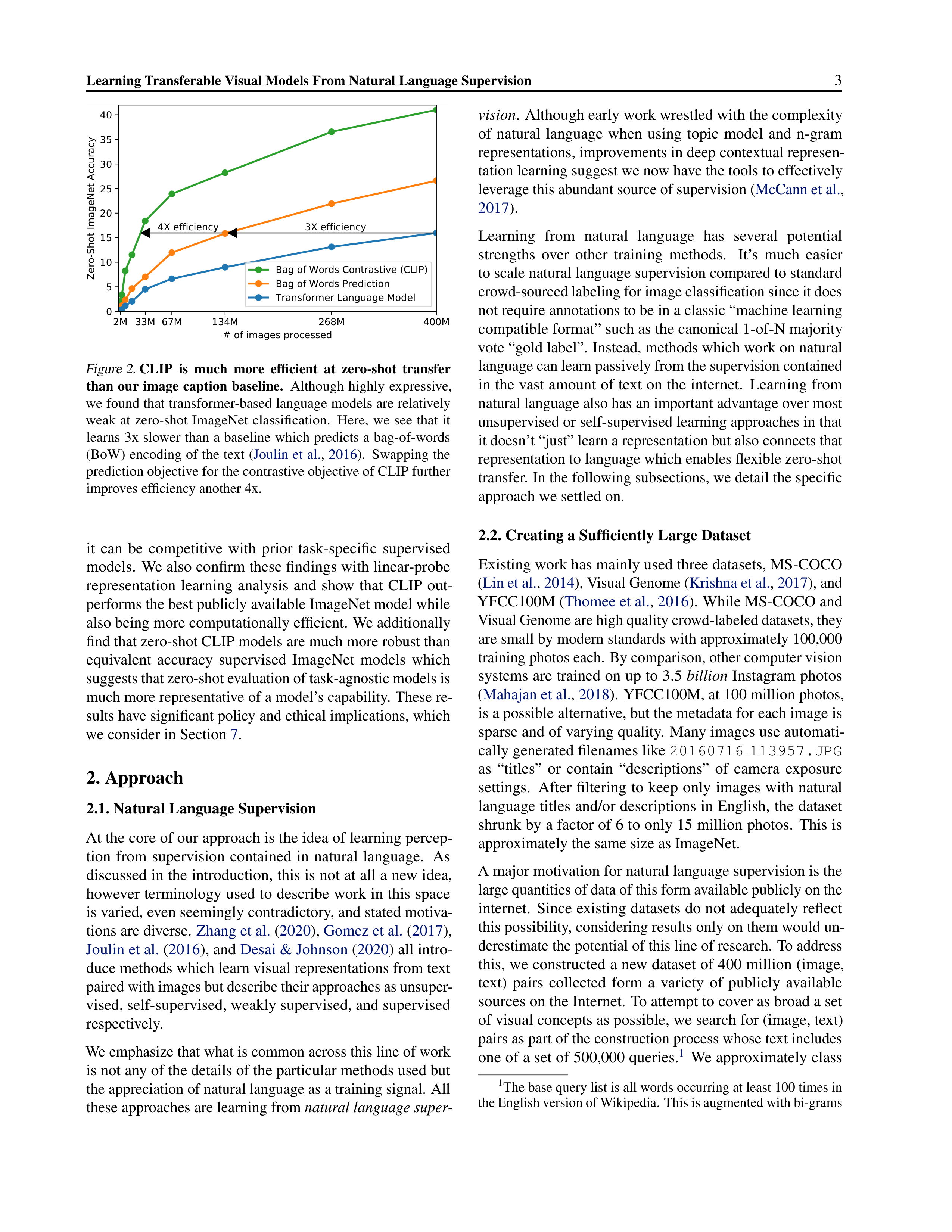
Figure 2.
CLIP
is
much
more
efficient
at
zero-shot
transfer
than
our
image
caption
baseline.
Although
highly
expressive,
we found that transformer-based language models are relatively
weak
at
zero-shot
ImageNet
classification.
Here,
we
see
that
it
learns
3x
slower
than
a
baseline
which
predicts
a
bag-of-words
(BoW) encoding of the text (
Joulin et al.
,
2016
).
Swapping the
prediction objective for the contrastive objective of CLIP further
improves efficiency another 4x.
it
can
be
competitive
with
prior
task-specific
supervised
models.
We also confirm these findings with linear-probe
representation
learning
analysis
and
show
that
CLIP
out-
performs the best publicly available ImageNet model while
also being more computationally efficient.
We additionally
find that zero-shot CLIP models are much more robust than
equivalent
accuracy
supervised
ImageNet
models
which
suggests that zero-shot evaluation of task-agnostic models is
much more representative of a model’s capability.
These re-
sults have significant policy and ethical implications, which
we consider in Section
7
.
2. Approach
2.1. Natural Language Supervision
At the core of our approach is the idea of learning percep-
tion
from
supervision
contained
in
natural
language.
As
discussed in the introduction, this is not at all a new idea,
however terminology used to describe work in this space
is varied, even seemingly contradictory, and stated motiva-
tions are diverse.
Zhang et al.
(
2020
),
Gomez et al.
(
2017
),
Joulin et al.
(
2016
), and
Desai & Johnson
(
2020
) all intro-
duce methods which learn visual representations from text
paired with images but describe their approaches as unsuper-
vised, self-supervised, weakly supervised, and supervised
respectively.
We emphasize that what is common across this line of work
is not any of the details of the particular methods used but
the appreciation of natural language as a training signal.
All
these approaches are learning from
natural language super-
vision
.
Although early work wrestled with the complexity
of
natural
language
when
using
topic
model
and
n-gram
representations, improvements in deep contextual represen-
tation learning suggest we now have the tools to effectively
leverage this abundant source of supervision (
McCann et al.
,
2017
).
Learning
from
natural
language
has
several
potential
strengths
over
other
training
methods.
It’s
much
easier
to scale natural language supervision compared to standard
crowd-sourced labeling for image classification since it does
not require annotations to be in a classic “machine learning
compatible format” such as the canonical 1-of-N majority
vote “gold label”.
Instead, methods which work on natural
language can learn passively from the supervision contained
in the vast amount of text on the internet.
Learning from
natural language also has an important advantage over most
unsupervised or self-supervised learning approaches in that
it doesn’t “just” learn a representation but also connects that
representation to language which enables flexible zero-shot
transfer.
In the following subsections, we detail the specific
approach we settled on.
2.2. Creating a Sufficiently Large Dataset
Existing work has mainly used three datasets, MS-COCO
(
Lin et al.
,
2014
), Visual Genome (
Krishna et al.
,
2017
), and
YFCC100M (
Thomee et al.
,
2016
).
While MS-COCO and
Visual Genome are high quality crowd-labeled datasets, they
are small by modern standards with approximately 100,000
training photos each.
By comparison, other computer vision
systems are trained on up to 3.5
billion
Instagram photos
(
Mahajan et al.
,
2018
).
YFCC100M, at 100 million photos,
is a possible alternative, but the metadata for each image is
sparse and of varying quality.
Many images use automati-
cally generated filenames like
20160716
113957.JPG
as
“titles”
or
contain
“descriptions”
of
camera
exposure
settings.
After
filtering
to
keep
only
images
with
natural
language titles and/or descriptions in English, the dataset
shrunk by a factor of 6 to only 15 million photos.
This is
approximately the same size as ImageNet.
A major motivation for natural language supervision is the
large quantities of data of this form available publicly on the
internet.
Since existing datasets do not adequately reflect
this possibility, considering results only on them would un-
derestimate the potential of this line of research.
To address
this, we constructed a new dataset of 400 million (image,
text)
pairs
collected
form
a
variety
of
publicly
available
sources on the Internet.
To attempt to cover as broad a set
of visual concepts as possible, we search for (image, text)
pairs as part of the construction process whose text includes
one of a set of 500,000 queries.
1
We approximately class
1
The base query list is all words occurring at least 100 times in
the English version of Wikipedia.
This is augmented with bi-grams
Learning Transferable Visual Models From Natural Language Supervision
4
balance the results by including up to 20,000 (image, text)
pairs
per
query.
The
resulting
dataset
has
a
similar
total
word count as the WebText dataset used to train GPT-2.
We
refer to this dataset as WIT for WebImageText.
2.3. Selecting an Efficient Pre-Training Method
State-of-the-art
computer
vision
systems
use
very
large
amounts
of
compute.
Mahajan
et
al.
(
2018
)
required
19
GPU years to train their ResNeXt101-32x48d and
Xie et al.
(
2020
) required 33 TPUv3 core-years to train their Noisy
Student EfficientNet-L2.
When considering that both these
systems were trained to predict only 1000 ImageNet classes,
the
task
of
learning
an
open
set
of
visual
concepts
from
natural language seems daunting.
In the course of our ef-
forts, we found training efficiency was key to successfully
scaling natural language supervision and we selected our
final pre-training method based on this metric.
Our initial approach,
similar to VirTex,
jointly trained an
image CNN and text transformer from scratch to predict the
caption of an image.
However, we encountered difficulties
efficiently scaling this method.
In Figure
2
we show that a
63 million parameter transformer language model, which
already
uses
twice
the
compute
of
its
ResNet-50
image
encoder, learns to recognize ImageNet classes three times
slower than a much simpler baseline that predicts a bag-of-
words encoding of the same text.
Both these approaches share a key similarity. They try to pre-
dict the
exact
words of the text accompanying each image.
This is a difficult task due to the wide variety of descriptions,
comments, and related text that co-occur with images.
Re-
cent work in contrastive representation learning for images
has found that contrastive objectives can learn better repre-
sentations than their equivalent predictive objective (
Tian
et al.
,
2019
).
Other work has found that although generative
models of images can learn high quality image representa-
tions, they require over an order of magnitude more compute
than contrastive models with the same performance (
Chen
et al.
,
2020a
).
Noting these findings, we explored training
a system to solve the potentially easier proxy task of pre-
dicting
only
which
text
as
a
whole
is
paired
with
which
image and not the exact words of that text.
Starting with
the same bag-of-words encoding baseline, we swapped the
predictive objective for a contrastive objective in Figure
2
and observed a further 4x efficiency improvement in the rate
of zero-shot transfer to ImageNet.
Given a batch of
N
(image, text) pairs, CLIP is trained to
predict which of the
N
×
N
possible (image, text) pairings
across a batch actually occurred.
To do this, CLIP learns a
with high pointwise mutual information as well as the names of
all Wikipedia articles above a certain search volume.
Finally all
WordNet synsets not already in the query list are added.
multi-modal embedding space by jointly training an image
encoder and text encoder to maximize the cosine similar-
ity
of
the
image
and
text
embeddings
of
the
N
real
pairs
in the batch while minimizing the cosine similarity of the
embeddings
of
the
N
2
−
N
incorrect
pairings.
We
opti-
mize a symmetric cross entropy loss over these similarity
scores.
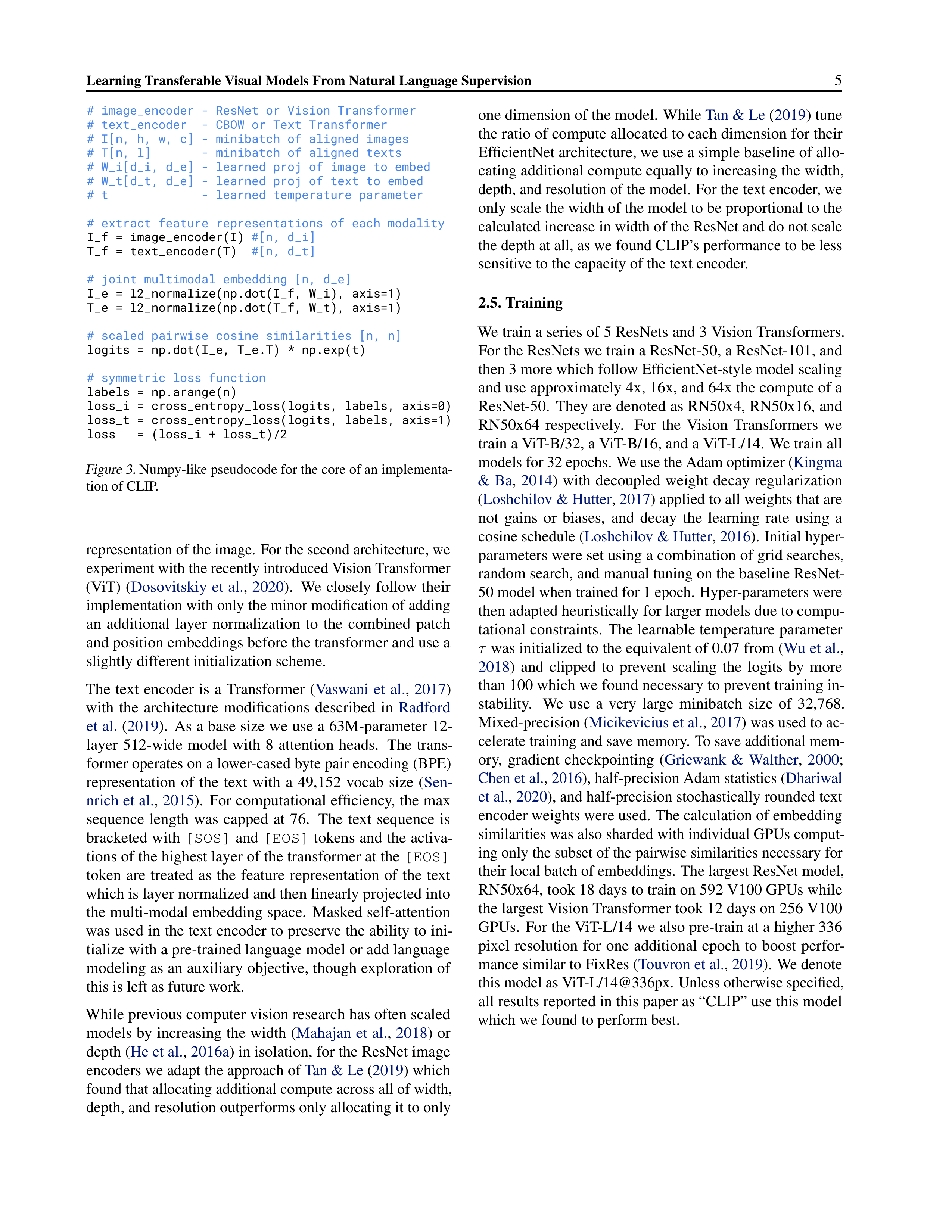
In Figure
3
we include pseudocode of the core of an
implementation of CLIP. To our knowledge this batch con-
struction technique and objective was first introduced in the
area of deep metric learning as the
multi-class N-pair loss
Sohn
(
2016
), was popularized for contrastive representation
learning by
Oord et al.
(
2018
) as the InfoNCE loss, and was
recently adapted for contrastive (text, image) representation
learning in the domain of medical imaging by
Zhang et al.
(
2020
).
Due to the large size of our pre-training dataset, over-fitting
is not a major concern and the details of training CLIP are
simplified compared to the implementation of
Zhang et al.
(
2020
).
We train CLIP from scratch without initializing the
image encoder with ImageNet weights or the text encoder
with
pre-trained
weights.
We
do
not
use
the
non-linear
projection between the representation and the contrastive
embedding space, a change which was introduced by
Bach-
man et al.
(
2019
) and popularized by
Chen et al.
(
2020b
).
We instead use only a linear projection to map from each en-
coder’s representation to the multi-modal embedding space.
We did not notice a difference in training efficiency between
the two versions and speculate that non-linear projections
may
be
co-adapted
with
details
of
current
image
only
in
self-supervised representation learning methods.
We also
remove the text transformation function
t
u
from
Zhang et al.
(
2020
)
which
samples
a
single
sentence
at
uniform
from
the text since many of the (image, text) pairs in CLIP’s pre-
training dataset are only a single sentence.
We also simplify
the
image
transformation
function
t
v
.
A
random
square
crop
from
resized
images
is
the
only
data
augmentation
used
during
training.
Finally,
the
temperature
parameter
which controls the range of the logits in the softmax,
τ
, is
directly optimized during training as a log-parameterized
multiplicative scalar to avoid turning as a hyper-parameter.
2.4. Choosing and Scaling a Model
We
consider
two
different
architectures
for
the
image
en-
coder.
For
the
first,
we
use
ResNet-50
(
He
et
al.
,
2016a
)
as
the
base
architecture
for
the
image
encoder
due
to
its
widespread adoption and proven performance. We make sev-
eral modifications to the original version using the ResNet-
D improvements from
He et al.
(
2019
) and the antialiased
rect-2
blur
pooling
from
Zhang
(
2019
).
We
also
replace
the global average pooling layer with an attention pooling
mechanism.
The attention pooling is implemented as a sin-
gle layer of “transformer-style” multi-head QKV attention
where the query is conditioned on the global average-pooled
Learning Transferable Visual Models From Natural Language Supervision
5
# image_encoder - ResNet or Vision Transformer
# text_encoder - CBOW or Text Transformer
# I[n, h, w, c] - minibatch of aligned images
# T[n, l] - minibatch of aligned texts
# W_i[d_i, d_e] - learned proj of image to embed
# W_t[d_t, d_e] - learned proj of text to embed
# t - learned temperature parameter
# extract feature representations of each modality
I_f = image_encoder(I)
#[n, d_i]
T_f = text_encoder(T)
#[n, d_t]
# joint multimodal embedding [n, d_e]
I_e = l2_normalize(np.dot(I_f, W_i), axis=1)
T_e = l2_normalize(np.dot(T_f, W_t), axis=1)
# scaled pairwise cosine similarities [n, n]
logits = np.dot(I_e, T_e.T) * np.exp(t)
# symmetric loss function
labels = np.arange(n)
loss_i = cross_entropy_loss(logits, labels, axis=0)
loss_t = cross_entropy_loss(logits, labels, axis=1)
loss = (loss_i + loss_t)/2
Figure 3.
Numpy-like pseudocode for the core of an implementa-
tion of CLIP.
representation of the image.
For the second architecture, we
experiment with the recently introduced Vision Transformer
(ViT)
(
Dosovitskiy
et
al.
,
2020
).
We
closely
follow
their
implementation with only the minor modification of adding
an
additional
layer
normalization
to
the
combined
patch
and position embeddings before the transformer and use a
slightly different initialization scheme.
The
text
encoder
is
a
Transformer
(
Vaswani
et
al.
,
2017
)
with
the
architecture
modifications
described
in
Radford
et al.
(
2019
).
As a base size we use a 63M-parameter 12-
layer
512-wide
model
with
8
attention
heads.
The
trans-
former operates on a lower-cased byte pair encoding (BPE)
representation
of
the
text
with
a
49,152
vocab
size
(
Sen-
nrich et al.
,
2015
).
For computational efficiency, the max
sequence
length
was
capped
at
76.
The
text
sequence
is
bracketed with
[SOS]
and
[EOS]
tokens and the activa-
tions of the highest layer of the transformer at the
[EOS]
token
are
treated
as
the
feature
representation
of
the
text
which is layer normalized and then linearly projected into
the multi-modal embedding space.
Masked self-attention
was used in the text encoder to preserve the ability to ini-
tialize with a pre-trained language model or add language
modeling as an auxiliary objective, though exploration of
this is left as future work.
While previous computer vision research has often scaled
models by increasing the width (
Mahajan et al.
,
2018
) or
depth (
He et al.
,
2016a
) in isolation, for the ResNet image
encoders we adapt the approach of
Tan & Le
(
2019
) which
found that allocating additional compute across all of width,
depth, and resolution outperforms only allocating it to only
one dimension of the model.
While
Tan & Le
(
2019
) tune
the ratio of compute allocated to each dimension for their
EfficientNet architecture, we use a simple baseline of allo-
cating additional compute equally to increasing the width,
depth, and resolution of the model.
For the text encoder, we
only scale the width of the model to be proportional to the
calculated increase in width of the ResNet and do not scale
the depth at all, as we found CLIP’s performance to be less
sensitive to the capacity of the text encoder.
2.5. Training
We train a series of 5 ResNets and 3 Vision Transformers.
For the ResNets we train a ResNet-50, a ResNet-101, and
then 3 more which follow EfficientNet-style model scaling
and use approximately 4x, 16x, and 64x the compute of a
ResNet-50.
They are denoted as RN50x4, RN50x16, and
RN50x64
respectively.
For
the
Vision
Transformers
we
train a ViT-B/32, a ViT-B/16, and a ViT-L/14.
We train all
models for 32 epochs.
We use the Adam optimizer (
Kingma
&
Ba
,
2014
)
with
decoupled
weight
decay
regularization
(
Loshchilov & Hutter
,
2017
) applied to all weights that are
not
gains
or
biases,
and
decay
the
learning
rate
using
a
cosine schedule (
Loshchilov & Hutter
,
2016
).
Initial hyper-
parameters were set using a combination of grid searches,
random search, and manual tuning on the baseline ResNet-
50 model when trained for 1 epoch.
Hyper-parameters were
then adapted heuristically for larger models due to compu-
tational constraints.
The learnable temperature parameter
τ
was initialized to the equivalent of 0.07 from (
Wu et al.
,
2018
)
and
clipped
to
prevent
scaling
the
logits
by
more
than 100 which we found necessary to prevent training in-
stability.
We
use
a
very
large
minibatch
size
of
32,768.
Mixed-precision (
Micikevicius et al.
,
2017
) was used to ac-
celerate training and save memory.
To save additional mem-
ory,
gradient
checkpointing
(
Griewank
&
Walther
,
2000
;
Chen et al.
,
2016
), half-precision Adam statistics (
Dhariwal
et al.
,
2020
), and half-precision stochastically rounded text
encoder weights were used.
The calculation of embedding
similarities was also sharded with individual GPUs comput-
ing only the subset of the pairwise similarities necessary for
their local batch of embeddings.
The largest ResNet model,
RN50x64, took 18 days to train on 592 V100 GPUs while
the largest Vision Transformer took 12 days on 256 V100
GPUs.
For the ViT-L/14 we also pre-train at a higher 336
pixel
resolution
for
one
additional
epoch
to
boost
perfor-
mance similar to FixRes (
Touvron et al.
,
2019
).
We denote
this model as ViT-L/14@336px.
Unless otherwise specified,
all results reported in this paper as “CLIP” use this model
which we found to perform best.
Learning Transferable Visual Models From Natural Language Supervision
6
3. Experiments
3.1. Zero-Shot Transfer
3.1.1. M
OTIVATION
In computer vision, zero-shot learning usually refers to the
study of generalizing to unseen object categories in image
classification
(
Lampert
et
al.
,
2009
).
We
instead
use
the
term in a broader sense and study generalization to unseen
datasets.
We
motivate
this
as
a
proxy
for
performing
un-
seen tasks, as aspired to in the zero-data learning paper of
Larochelle et al.
(
2008
).
While much research in the field of
unsupervised learning focuses on the
representation learn-
ing
capabilities of machine learning systems, we motivate
studying zero-shot transfer as a way of measuring the
task-
learning
capabilities of machine learning systems.
In this
view,
a
dataset
evaluates
performance
on
a
task
on
a
spe-
cific distribution.
However, many popular computer vision
datasets were created by the research community primarily
as benchmarks to guide the development of generic image
classification methods rather than measuring performance
on
a
specific
task.
While
it
is
reasonable
to
say
that
the
SVHN dataset measures the task of street number transcrip-
tion on the distribution of Google Street View photos, it is
unclear
what
“real”
task
the
CIFAR-10
dataset
measures.
It is clear, however, what distribution CIFAR-10 is drawn
from - TinyImages (
Torralba et al.
,
2008
).
On these kinds of
datasets, zero-shot transfer is more an evaluation of CLIP’s
robustness to distribution shift and domain generalization
rather than task generalization.
Please see Section
3.3
for
analysis focused on this.
To
our
knowledge,
Visual
N-Grams
(
Li
et
al.
,
2017
)
first
studied zero-shot transfer to existing image classification
datasets in the manner described above.
It is also the only
other work we are aware of that has studied zero-shot trans-
fer to standard image classification datasets using a gener-
ically
pre-trained
model
and
serves
as
the
best
reference
point for contextualizing CLIP. Their approach learns the
parameters of a dictionary of 142,806 visual n-grams (span-
ning 1- to 5- grams) and optimizes these n-grams using a
differential version of Jelinek-Mercer smoothing to maxi-
mize the probability of all text n-grams for a given image.
In order to perform zero-shot transfer, they first convert the
text
of
each
of
the
dataset’s
class
names
into
its
n-gram
representation and then compute its probability according
to their model, predicting the one with the highest score.
Our focus on studying zero-shot transfer as an evaluation of
task learning is inspired by work demonstrating task learn-
ing in the field of NLP. To our knowledge
Liu et al.
(
2018
)
first identified task learning as an “unexpected side-effect”
when a language model trained to generate Wikipedia ar-
ticles
learned
to
reliably
transliterate
names
between
lan-
guages.
While GPT-1 (
Radford et al.
,
2018
) focused on pre-
training as a transfer learning method to improve supervised
fine-tuning, it also included an ablation study demonstrat-
ing that the performance of four heuristic zero-shot transfer
methods improved steadily over the course of pre-training,
without any supervised adaption.
This analysis served as the
basis for GPT-2 (
Radford et al.
,
2019
) which focused exclu-
sively on studying the task-learning capabilities of language
models via zero-shot transfer.
3.1.2. U
SING
CLIP
FOR
Z
ERO
-S
HOT
T
RANSFER
CLIP is pre-trained to predict if an image and a text snippet
are paired together in its dataset.
To perform zero-shot clas-
sification, we reuse this capability.
For each dataset, we use
the names of all the classes in the dataset as the set of poten-
tial text pairings and predict the most probable (image, text)
pair according to CLIP. In a bit more detail, we first compute
the feature embedding of the image and the feature embed-
ding of the set of possible texts by their respective encoders.
The cosine similarity of these embeddings is then calculated,
scaled by a temperature parameter
τ
, and normalized into a
probability distribution via a softmax.
Note that this predic-
tion layer is a multinomial logistic regression classifier with
L2-normalized inputs, L2-normalized weights, no bias, and
temperature scaling.
When interpreted this way, the image
encoder is the computer vision backbone which computes a
feature representation for the image and the text encoder is a
hypernetwork (
Ha et al.
,
2016
) which generates the weights
of a linear classifier based on the text specifying the visual
concepts that the classes represent.
Lei Ba et al.
(
2015
) first
introduced a zero-shot image classifier of this form while
the
idea
of
generating
a
classifier
from
natural
language
dates back to at least
Elhoseiny et al.
(
2013
).
Continuing
with this interpretation, every step of CLIP pre-training can
be
viewed
as
optimizing
the
performance
of
a
randomly
created proxy to a computer vision dataset which contains 1
example per class and has 32,768 total classes defined via
natural language descriptions.
For zero-shot evaluation, we
cache the zero-shot classifier once it has been computed by
the text encoder and reuse it for all subsequent predictions.
This allows the cost of generating it to be amortized across
all the predictions in a dataset.
3.1.3. I
NITIAL
C
OMPARISON
TO
V
ISUAL
N-G
RAMS
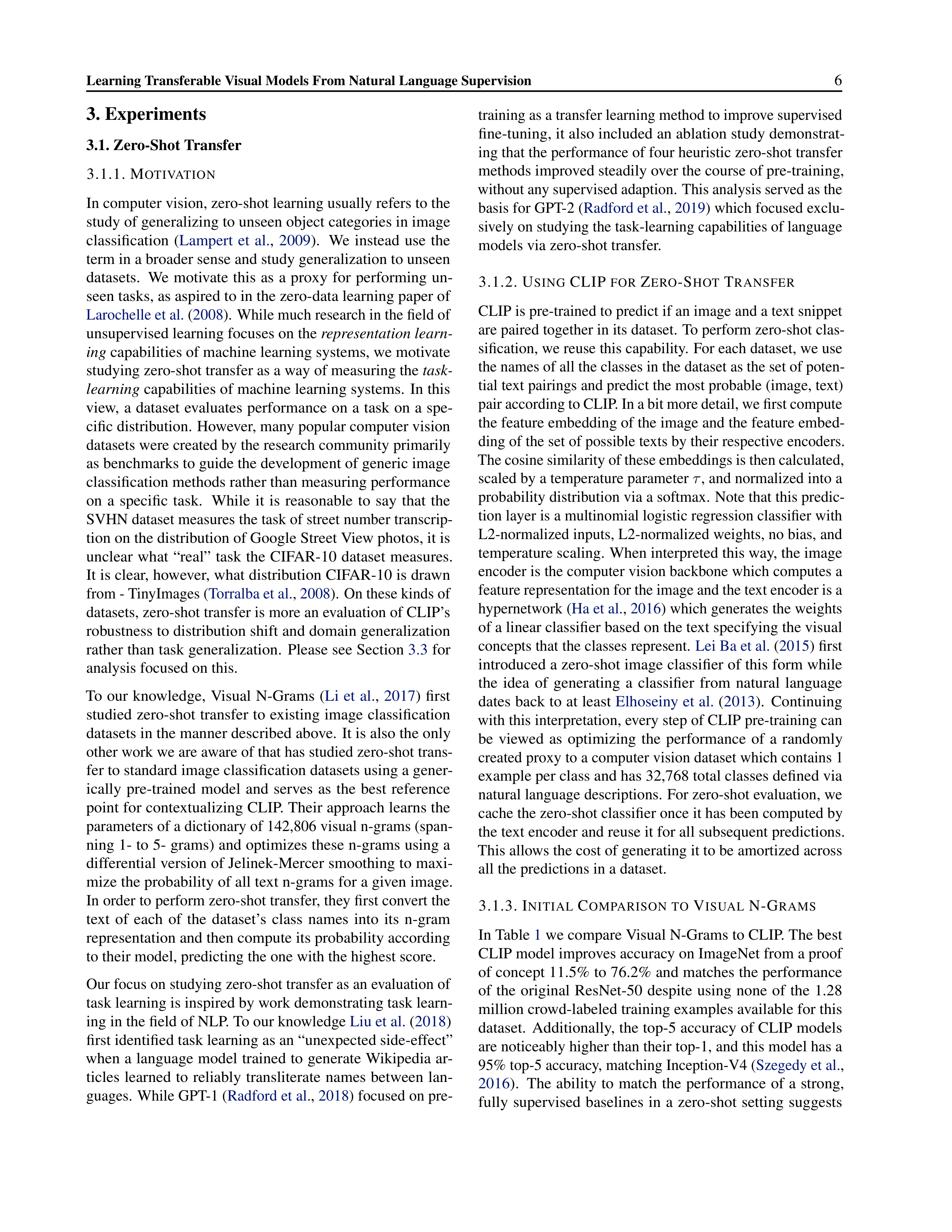
In Table
1
we compare Visual N-Grams to CLIP. The best
CLIP model improves accuracy on ImageNet from a proof
of concept 11.5% to 76.2% and matches the performance
of
the
original
ResNet-50
despite
using
none
of
the
1.28
million crowd-labeled training examples available for this
dataset.
Additionally, the top-5 accuracy of CLIP models
are noticeably higher than their top-1, and this model has a
95% top-5 accuracy, matching Inception-V4 (
Szegedy et al.
,
2016
).
The
ability
to
match
the
performance
of
a
strong,
fully
supervised
baselines
in
a
zero-shot
setting
suggests
Learning Transferable Visual Models From Natural Language Supervision
7
aYahoo
ImageNet
SUN
Visual N-Grams
72.4
11.5
23.0
CLIP
98.4
76.2
58.5
Table 1.
Comparing CLIP to prior zero-shot transfer image classi-
fication results.
CLIP improves performance on all three datasets
by a large amount.
This improvement reflects many differences
in the 4 years since the development of Visual N-Grams (
Li et al.
,
2017
).
CLIP
is
a
significant
step
towards
flexible
and
practical
zero-shot computer vision classifiers.
As mentioned above,
the comparison to Visual N-Grams is meant for contextu-
alizing
the
performance
of
CLIP
and
should
not
be
inter-
preted as a direct methods comparison between CLIP and
Visual N-Grams as many performance relevant differences
between
the
two
systems
were
not
controlled
for.
For
in-
stance, we train on a dataset that is 10x larger, use a vision
model that requires nearly 100x more compute per predic-
tion,
likely
used
over
1000x
their
training
compute,
and
use
a
transformer-based
model
which
did
not
exist
when
Visual N-Grams was published.
As a closer comparison, we
trained a CLIP ResNet-50 on the same YFCC100M dataset
that Visual N-Grams was trained on and found it matched
their reported ImageNet performance within a V100 GPU
day.
This baseline was also trained from scratch instead of
being initialized from pre-trained ImageNet weights as in
Visual N-Grams.
CLIP also outperforms Visual N-Grams on the other 2 re-
ported datasets.
On aYahoo, CLIP achieves a 95% reduction
in the number of errors, and on SUN, CLIP more than dou-
bles the accuracy of Visual N-Grams.
To conduct a more
comprehensive
analysis
and
stress
test,
we
implement
a
much
larger
evaluation
suite
detailed
in
Appendix
A
.
In
total we expand from the 3 datasets reported in Visual N-
Grams to include over 30 datasets and compare to over 50
existing computer vision systems to contextualize results.
3.1.4. P
ROMPT
E
NGINEERING
AND
E
NSEMBLING
Most standard image classification datasets treat the infor-
mation naming or describing classes which enables natural
language based zero-shot transfer as an afterthought.
The
vast majority of datasets annotate images with just a numeric
id of the label and contain a file mapping these ids back to
their names in English.
Some datasets, such as Flowers102
and
GTSRB,
don’t
appear
to
include
this
mapping
at
all
in their released versions preventing zero-shot transfer en-
tirely.
2
For many datasets, we observed these labels may be
2
Alec
learned
much
more
about
flower
species
and
German
traffic signs over the course of this project than he originally antic-
ipated.
6.1
9.9
21.5
75.3
265.9
Model GFLOPs
45
50
55
60
65
70
Average Score (%)
4X efficiency gain
5 point
improvement
RN50
RN101
RN50x4
RN50x16
RN50x64
Prompt engineering and ensembling
Contextless class names (Li et al. 2017)
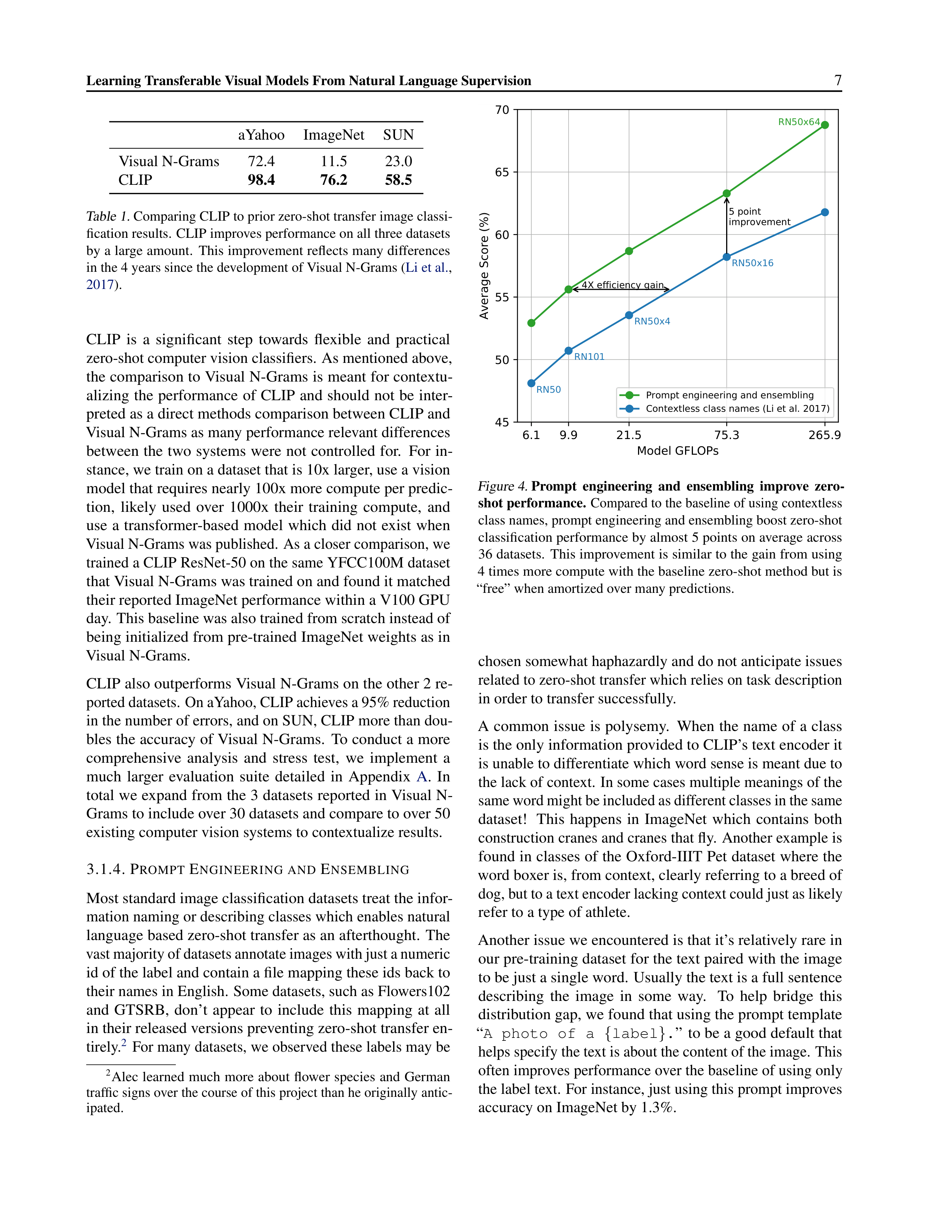
Figure 4.
Prompt
engineering
and
ensembling
improve
zero-
shot performance.
Compared to the baseline of using contextless
class names, prompt engineering and ensembling boost zero-shot
classification performance by almost 5 points on average across
36 datasets.
This improvement is similar to the gain from using
4 times more compute with the baseline zero-shot method but is
“free” when amortized over many predictions.
chosen somewhat haphazardly and do not anticipate issues
related to zero-shot transfer which relies on task description
in order to transfer successfully.
A common issue is polysemy.
When the name of a class
is the only information provided to CLIP’s text encoder it
is unable to differentiate which word sense is meant due to
the lack of context.
In some cases multiple meanings of the
same word might be included as different classes in the same
dataset!
This
happens
in
ImageNet
which
contains
both
construction cranes and cranes that fly.
Another example is
found in classes of the Oxford-IIIT Pet dataset where the
word boxer is, from context, clearly referring to a breed of
dog, but to a text encoder lacking context could just as likely
refer to a type of athlete.
Another issue we encountered is that it’s relatively rare in
our pre-training dataset for the text paired with the image
to be just a single word.
Usually the text is a full sentence
describing
the
image
in
some
way.
To
help
bridge
this
distribution gap, we found that using the prompt template
“
A
photo
of
a
{
label
}
.
”
to be a good default that
helps specify the text is about the content of the image.
This
often improves performance over the baseline of using only
the label text.
For instance, just using this prompt improves
accuracy on ImageNet by 1.3%.
Learning Transferable Visual Models From Natural Language Supervision
8
Similar to the “prompt engineering” discussion around GPT-
3
(
Brown
et
al.
,
2020
;
Gao
et
al.
,
2020
),
we
have
also
observed
that
zero-shot
performance
can
be
significantly
improved by customizing the prompt text to each task.
A
few, non exhaustive, examples follow.
We found on several
fine-grained image classification datasets that it helped to
specify the category.
For example on Oxford-IIIT Pets, us-
ing “
A
photo
of
a
{
label
}
,
a
type
of
pet.
”
to help provide context worked well.
Likewise, on Food101
specifying
a type of food
and on FGVC Aircraft
a type of
aircraft
helped too.
For OCR datasets, we found that putting
quotes around the text or number to be recognized improved
performance. Finally, we found that on satellite image classi-
fication datasets it helped to specify that the images were of
this form and we use variants of “
a
satellite
photo
of
a
{
label
}
.
”.
We also experimented with ensembling over multiple zero-
shot classifiers as another way of improving performance.
These classifiers are computed by using different context
prompts such as ‘
A
photo
of
a
big
{
label
}
” and
“
A
photo
of
a
small
{
label
}
”.
We construct the
ensemble over the embedding space instead of probability
space.
This allows us to cache a single set of averaged text
embeddings so that the compute cost of the ensemble is the
same as using a single classifier when amortized over many
predictions.
We’ve observed ensembling across many gen-
erated zero-shot classifiers to reliably improve performance
and use it for the majority of datasets.
On ImageNet,
we
ensemble 80 different context prompts and this improves
performance by an additional 3.5% over the single default
prompt discussed above.
When considered together, prompt
engineering
and
ensembling
improve
ImageNet
accuracy
by almost 5%.
In Figure
4
we visualize how prompt engi-
neering and ensembling change the performance of a set of
CLIP models compared to the contextless baseline approach
of
directly
embedding
the
class
name
as
done
in
Li
et
al.
(
2017
).
3.1.5. A
NALYSIS
OF
Z
ERO
-S
HOT
CLIP
P
ERFORMANCE
Since task-agnostic zero-shot classifiers for computer vision
have been understudied, CLIP provides a promising oppor-
tunity to gain a better understanding of this type of model.
In this section, we conduct a study of various properties of
CLIP’s
zero-shot
classifiers.
As
a
first
question,
we
look
simply at how well zero-shot classifiers perform.
To con-
textualize this, we compare to the performance of a simple
off-the-shelf baseline:
fitting a fully supervised, regularized,
logistic regression classifier on the features of the canonical
ResNet-50.
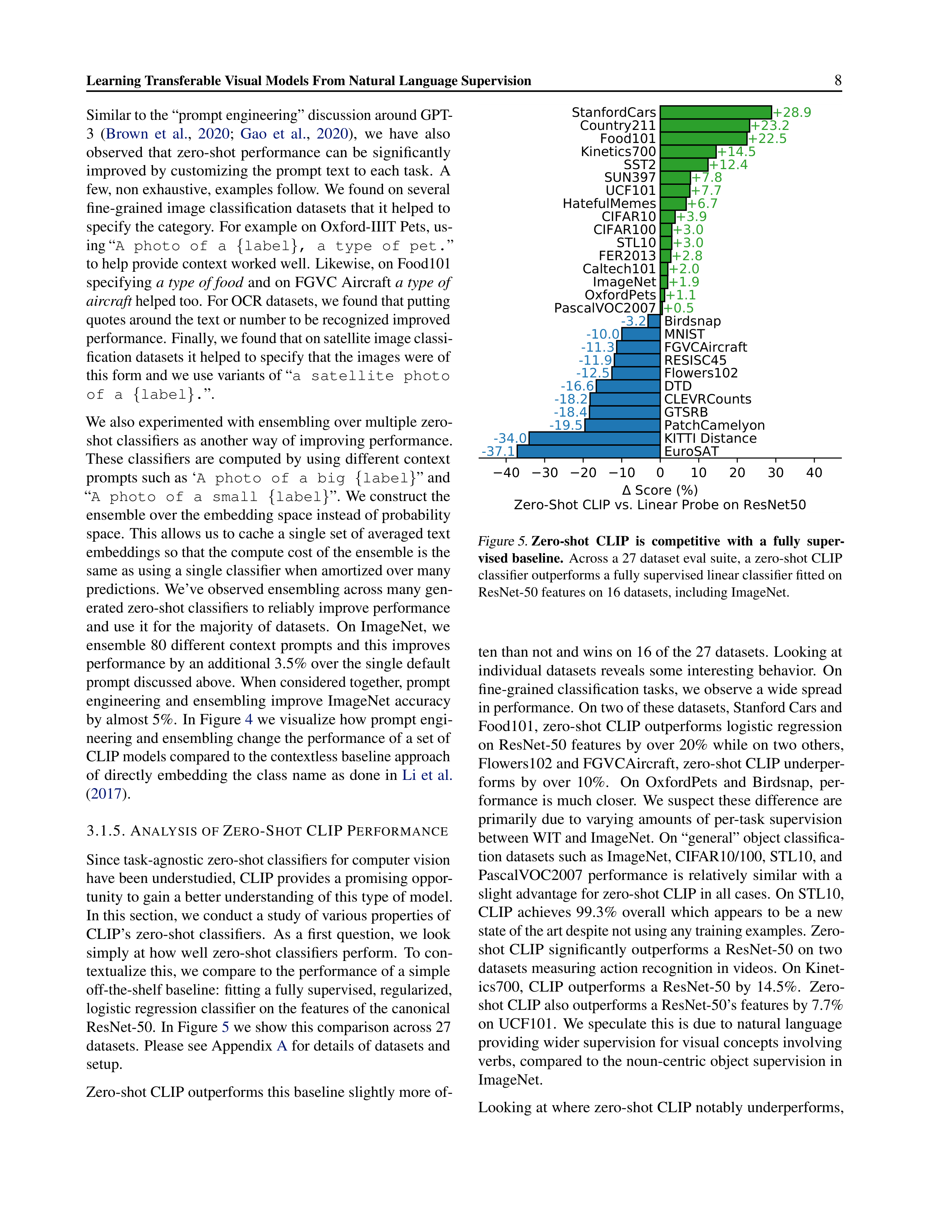
In Figure
5
we show this comparison across 27
datasets.
Please see Appendix
A
for details of datasets and
setup.
Zero-shot CLIP outperforms this baseline slightly more of-
40
30
20
10
0
10
20
30
40
Score (%)
Zero-Shot CLIP vs. Linear Probe on ResNet50
EuroSAT
-37.1
KITTI Distance
-34.0
PatchCamelyon
-19.5
GTSRB
-18.4
CLEVRCounts
-18.2
DTD
-16.6
Flowers102
-12.5
RESISC45
-11.9
FGVCAircraft
-11.3
MNIST
-10.0
Birdsnap
-3.2
+0.5
PascalVOC2007
+1.1
OxfordPets
+1.9
ImageNet
+2.0
Caltech101
+2.8
FER2013
+3.0
STL10
+3.0
CIFAR100
+3.9
CIFAR10
+6.7
HatefulMemes
+7.7
UCF101
+7.8
SUN397
+12.4
SST2
+14.5
Kinetics700
+22.5
Food101
+23.2
Country211
+28.9
StanfordCars
Figure 5.
Zero-shot
CLIP
is
competitive
with
a
fully
super-
vised baseline.
Across a 27 dataset eval suite, a zero-shot CLIP
classifier outperforms a fully supervised linear classifier fitted on
ResNet-50 features on 16 datasets, including ImageNet.
ten than not and wins on 16 of the 27 datasets.
Looking at
individual datasets reveals some interesting behavior.
On
fine-grained classification tasks, we observe a wide spread
in performance.
On two of these datasets, Stanford Cars and
Food101, zero-shot CLIP outperforms logistic regression
on
ResNet-50
features
by
over
20%
while
on
two
others,
Flowers102 and FGVCAircraft, zero-shot CLIP underper-
forms
by
over
10%.
On
OxfordPets
and
Birdsnap,
per-
formance is much closer.
We suspect these difference are
primarily due to varying amounts of per-task supervision
between WIT and ImageNet.
On “general” object classifica-
tion datasets such as ImageNet, CIFAR10/100, STL10, and
PascalVOC2007
performance
is
relatively
similar
with
a
slight advantage for zero-shot CLIP in all cases.
On STL10,
CLIP
achieves
99.3%
overall
which
appears
to
be
a
new
state of the art despite not using any training examples. Zero-
shot
CLIP
significantly
outperforms
a
ResNet-50
on
two
datasets measuring action recognition in videos.
On Kinet-
ics700,
CLIP
outperforms
a
ResNet-50
by
14.5%.
Zero-
shot CLIP also outperforms a ResNet-50’s features by 7.7%
on UCF101.
We speculate this is due to natural language
providing wider supervision for visual concepts involving
verbs, compared to the noun-centric object supervision in
ImageNet.
Looking at where zero-shot CLIP notably underperforms,
Learning Transferable Visual Models From Natural Language Supervision
9
0
1
2
4
8
16
# of labeled training examples per class
30
35
40
45
50
55
60
65
70
75
Average Score (%)
Zero-Shot
CLIP
BiT-M (ImageNet-21K)
Linear Probe CLIP
SimCLRv2
ResNet50
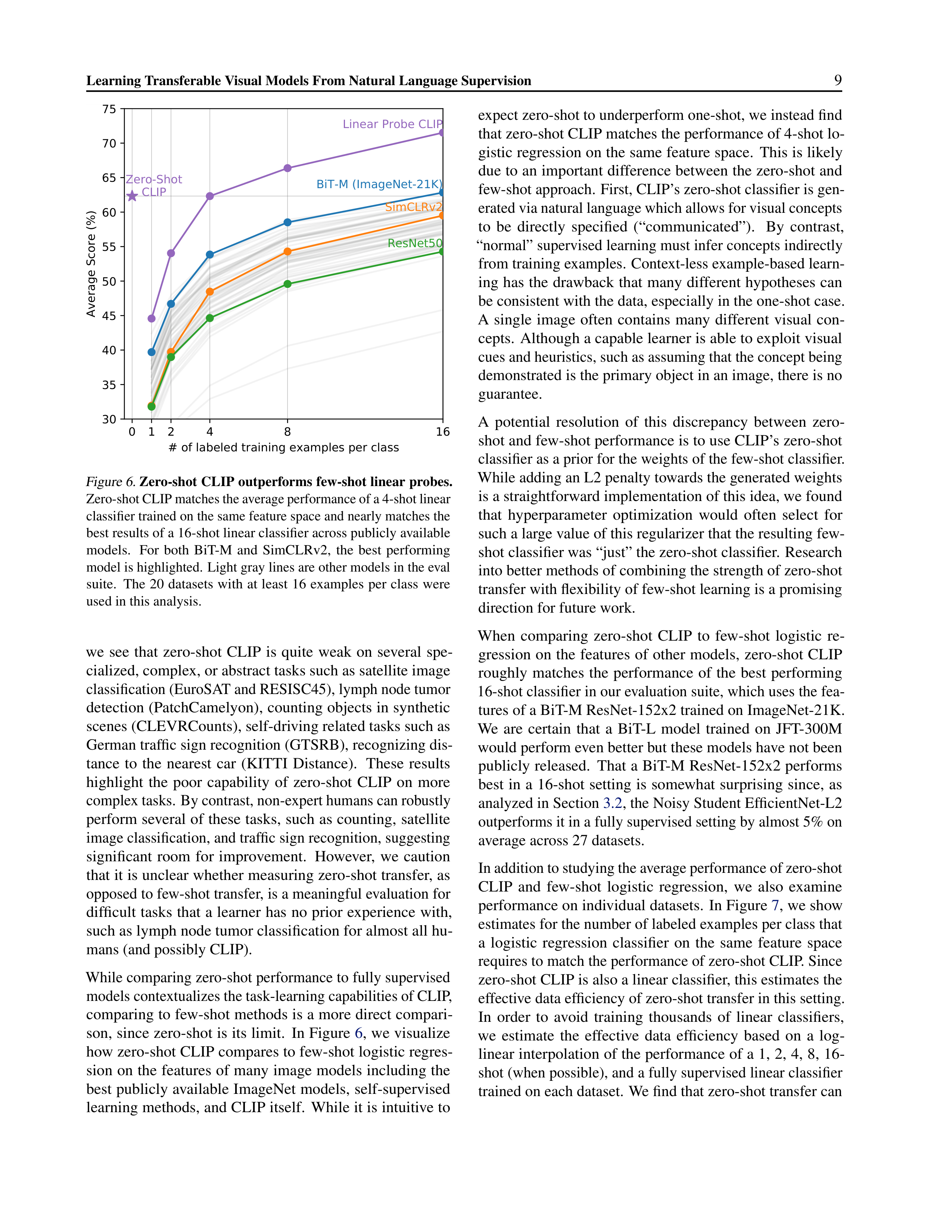
Figure 6.
Zero-shot CLIP outperforms few-shot linear probes.
Zero-shot CLIP matches the average performance of a 4-shot linear
classifier trained on the same feature space and nearly matches the
best results of a 16-shot linear classifier across publicly available
models.
For
both
BiT-M
and
SimCLRv2,
the
best
performing
model is highlighted.
Light gray lines are other models in the eval
suite.
The
20
datasets
with
at
least
16
examples
per
class
were
used in this analysis.
we
see
that
zero-shot
CLIP
is
quite
weak
on
several
spe-
cialized, complex, or abstract tasks such as satellite image
classification (EuroSAT and RESISC45), lymph node tumor
detection (PatchCamelyon), counting objects in synthetic
scenes (CLEVRCounts), self-driving related tasks such as
German traffic sign recognition (GTSRB), recognizing dis-
tance
to
the
nearest
car
(KITTI
Distance).
These
results
highlight
the
poor
capability
of
zero-shot
CLIP
on
more
complex tasks.
By contrast, non-expert humans can robustly
perform several of these tasks,
such as counting,
satellite
image classification, and traffic sign recognition, suggesting
significant
room
for
improvement.
However,
we
caution
that it is unclear whether measuring zero-shot transfer, as
opposed to few-shot transfer, is a meaningful evaluation for
difficult tasks that a learner has no prior experience with,
such as lymph node tumor classification for almost all hu-
mans (and possibly CLIP).
While comparing zero-shot performance to fully supervised
models contextualizes the task-learning capabilities of CLIP,
comparing to few-shot methods is a more direct compari-
son, since zero-shot is its limit.
In Figure
6
, we visualize
how zero-shot CLIP compares to few-shot logistic regres-
sion on the features of many image models including the
best publicly available ImageNet models, self-supervised
learning methods, and CLIP itself.
While it is intuitive to
expect zero-shot to underperform one-shot, we instead find
that zero-shot CLIP matches the performance of 4-shot lo-
gistic regression on the same feature space.
This is likely
due to an important difference between the zero-shot and
few-shot approach.
First, CLIP’s zero-shot classifier is gen-
erated via natural language which allows for visual concepts
to
be
directly
specified
(“communicated”).
By
contrast,
“normal” supervised learning must infer concepts indirectly
from training examples.
Context-less example-based learn-
ing has the drawback that many different hypotheses can
be consistent with the data, especially in the one-shot case.
A
single
image
often
contains
many
different
visual
con-
cepts.
Although a capable learner is able to exploit visual
cues and heuristics, such as assuming that the concept being
demonstrated is the primary object in an image, there is no
guarantee.
A
potential
resolution
of
this
discrepancy
between
zero-
shot and few-shot performance is to use CLIP’s zero-shot
classifier as a prior for the weights of the few-shot classifier.
While adding an L2 penalty towards the generated weights
is a straightforward implementation of this idea, we found
that
hyperparameter
optimization
would
often
select
for
such a large value of this regularizer that the resulting few-
shot classifier was “just” the zero-shot classifier.
Research
into better methods of combining the strength of zero-shot
transfer with flexibility of few-shot learning is a promising
direction for future work.
When
comparing
zero-shot
CLIP
to
few-shot
logistic
re-
gression on
the features
of other models,
zero-shot CLIP
roughly
matches
the
performance
of
the
best
performing
16-shot classifier in our evaluation suite, which uses the fea-
tures of a BiT-M ResNet-152x2 trained on ImageNet-21K.
We
are
certain
that
a
BiT-L
model
trained
on
JFT-300M
would perform even better but these models have not been
publicly released.
That a BiT-M ResNet-152x2 performs
best
in a
16-shot
setting is
somewhat
surprising
since,
as
analyzed in Section
3.2
, the Noisy Student EfficientNet-L2
outperforms it in a fully supervised setting by almost 5% on
average across 27 datasets.
In addition to studying the average performance of zero-shot
CLIP
and
few-shot
logistic
regression,
we
also
examine
performance on individual datasets.
In Figure
7
, we show
estimates for the number of labeled examples per class that
a
logistic
regression
classifier
on
the
same
feature
space
requires to match the performance of zero-shot CLIP. Since
zero-shot CLIP is also a linear classifier, this estimates the
effective data efficiency of zero-shot transfer in this setting.
In
order
to
avoid
training
thousands
of
linear
classifiers,
we
estimate
the
effective
data
efficiency
based
on
a
log-
linear interpolation of the performance of a 1, 2, 4, 8, 16-
shot (when possible), and a fully supervised linear classifier
trained on each dataset.
We find that zero-shot transfer can
Learning Transferable Visual Models From Natural Language Supervision
10
0
25
50
75
100
125
150
175
200
# of labeled examples per class
required to match zero-shot
Flowers102
EuroSAT
RESISC45
CLEVRCounts
GTSRB
FGVCAircraft
DTD
Birdsnap
UCF101
KITTI Distance
Caltech101
SUN397
MNIST
StanfordCars
HatefulMemes
CIFAR100
STL10
Kinetics700
SST2
PCam
ImageNet
Country211
OxfordPets
Food101
CIFAR10
FER2013
0.9
0.9
1.5
1.5
1.6
2.0
2.6
2.7
2.9
2.9
3.5
3.9
4.8
6.0
9.8
12.0
12.7
13.6
14.4
14.7
16.0
32
48
64
81
184
Median: 5.4
Mean: 20.8
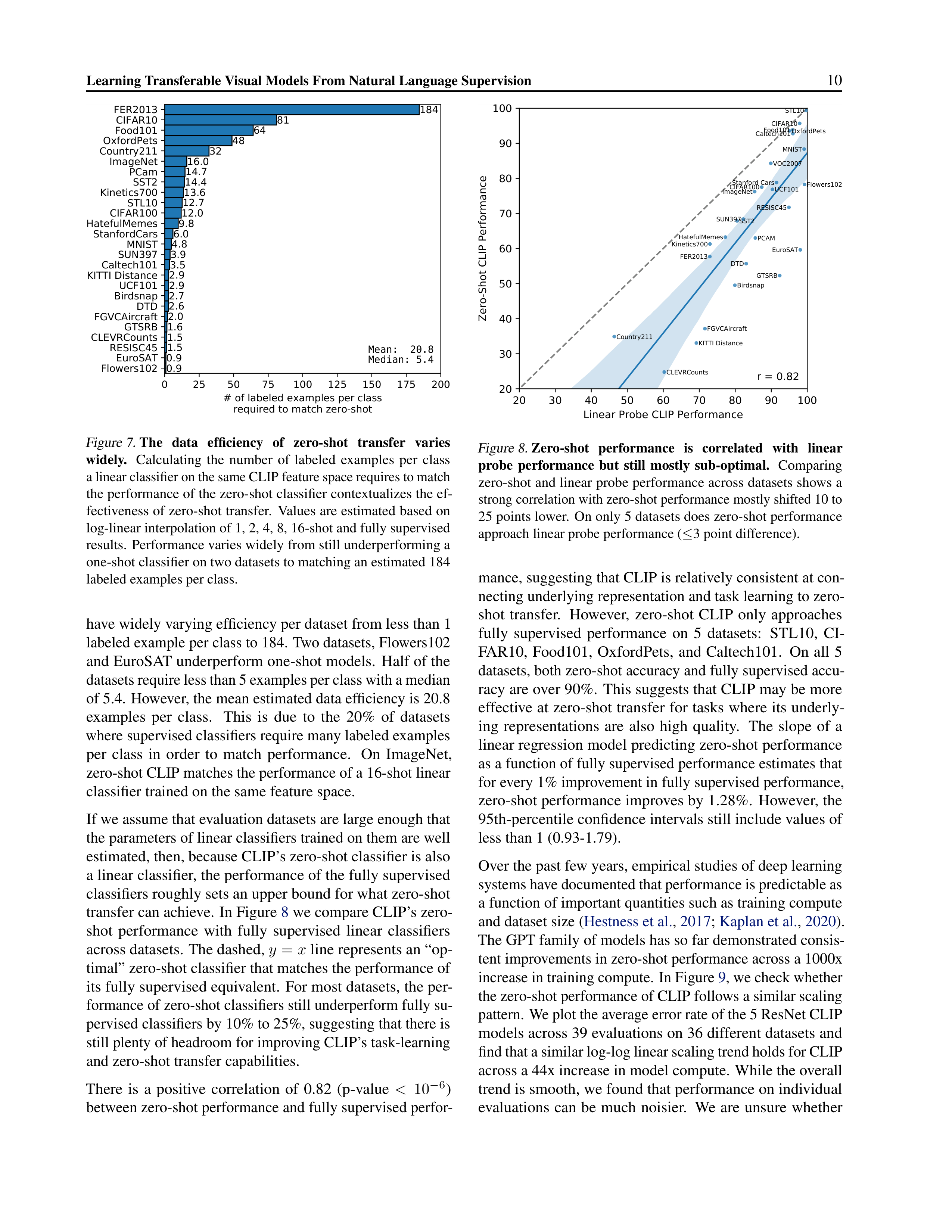
Figure 7.
The
data
efficiency
of
zero-shot
transfer
varies
widely.
Calculating
the
number
of
labeled
examples
per
class
a linear classifier on the same CLIP feature space requires to match
the performance of the zero-shot classifier contextualizes the ef-
fectiveness of zero-shot transfer.
Values are estimated based on
log-linear interpolation of 1, 2, 4, 8, 16-shot and fully supervised
results.
Performance varies widely from still underperforming a
one-shot classifier on two datasets to matching an estimated 184
labeled examples per class.
have widely varying efficiency per dataset from less than 1
labeled example per class to 184.
Two datasets, Flowers102
and EuroSAT underperform one-shot models.
Half of the
datasets require less than 5 examples per class with a median
of 5.4.
However, the mean estimated data efficiency is 20.8
examples
per
class.
This
is
due
to
the
20%
of
datasets
where supervised classifiers require many labeled examples
per
class
in
order
to
match
performance.
On
ImageNet,
zero-shot CLIP matches the performance of a 16-shot linear
classifier trained on the same feature space.
If we assume that evaluation datasets are large enough that
the parameters of linear classifiers trained on them are well
estimated, then, because CLIP’s zero-shot classifier is also
a linear classifier, the performance of the fully supervised
classifiers roughly sets an upper bound for what zero-shot
transfer can achieve.
In Figure
8
we compare CLIP’s zero-
shot
performance
with
fully
supervised
linear
classifiers
across datasets.
The dashed,
y
=
x
line represents an “op-
timal” zero-shot classifier that matches the performance of
its fully supervised equivalent.
For most datasets, the per-
formance of zero-shot classifiers still underperform fully su-
pervised classifiers by 10% to 25%, suggesting that there is
still plenty of headroom for improving CLIP’s task-learning
and zero-shot transfer capabilities.
There
is
a
positive
correlation
of
0.82
(p-value
<
10
−
6
)
between zero-shot performance and fully supervised perfor-
20
30
40
50
60
70
80
90
100
Linear Probe CLIP Performance
20
30
40
50
60
70
80
90
100
Zero-Shot CLIP Performance
r = 0.82
VOC2007
Country211
HatefulMemes
MNIST
CIFAR10
SST2
DTD
PCAM
RESISC45
EuroSAT
GTSRB
CLEVRCounts
FER2013
UCF101
Birdsnap
OxfordPets
CIFAR100
FGVCAircraft
Food101
Flowers102
Stanford Cars
Caltech101
SUN397
ImageNet
STL10
KITTI Distance
Kinetics700
Figure 8.
Zero-shot
performance
is
correlated
with
linear
probe
performance
but
still
mostly
sub-optimal.
Comparing
zero-shot and linear probe performance across datasets shows a
strong correlation with zero-shot performance mostly shifted 10 to
25 points lower.
On only 5 datasets does zero-shot performance
approach linear probe performance (
≤
3 point difference).
mance, suggesting that CLIP is relatively consistent at con-
necting underlying representation and task learning to zero-
shot
transfer.
However,
zero-shot
CLIP
only
approaches
fully
supervised
performance
on
5
datasets:
STL10,
CI-
FAR10,
Food101,
OxfordPets,
and
Caltech101.
On
all
5
datasets, both zero-shot accuracy and fully supervised accu-
racy are over 90%.
This suggests that CLIP may be more
effective at zero-shot transfer for tasks where its underly-
ing
representations
are
also
high
quality.
The
slope
of
a
linear regression model predicting zero-shot performance
as a function of fully supervised performance estimates that
for every 1% improvement in fully supervised performance,
zero-shot performance improves by 1.28%.
However, the
95th-percentile confidence intervals still include values of
less than 1 (0.93-1.79).
Over the past few years, empirical studies of deep learning
systems have documented that performance is predictable as
a function of important quantities such as training compute
and dataset size (
Hestness et al.
,
2017
;
Kaplan et al.
,
2020
).
The GPT family of models has so far demonstrated consis-
tent improvements in zero-shot performance across a 1000x
increase in training compute.
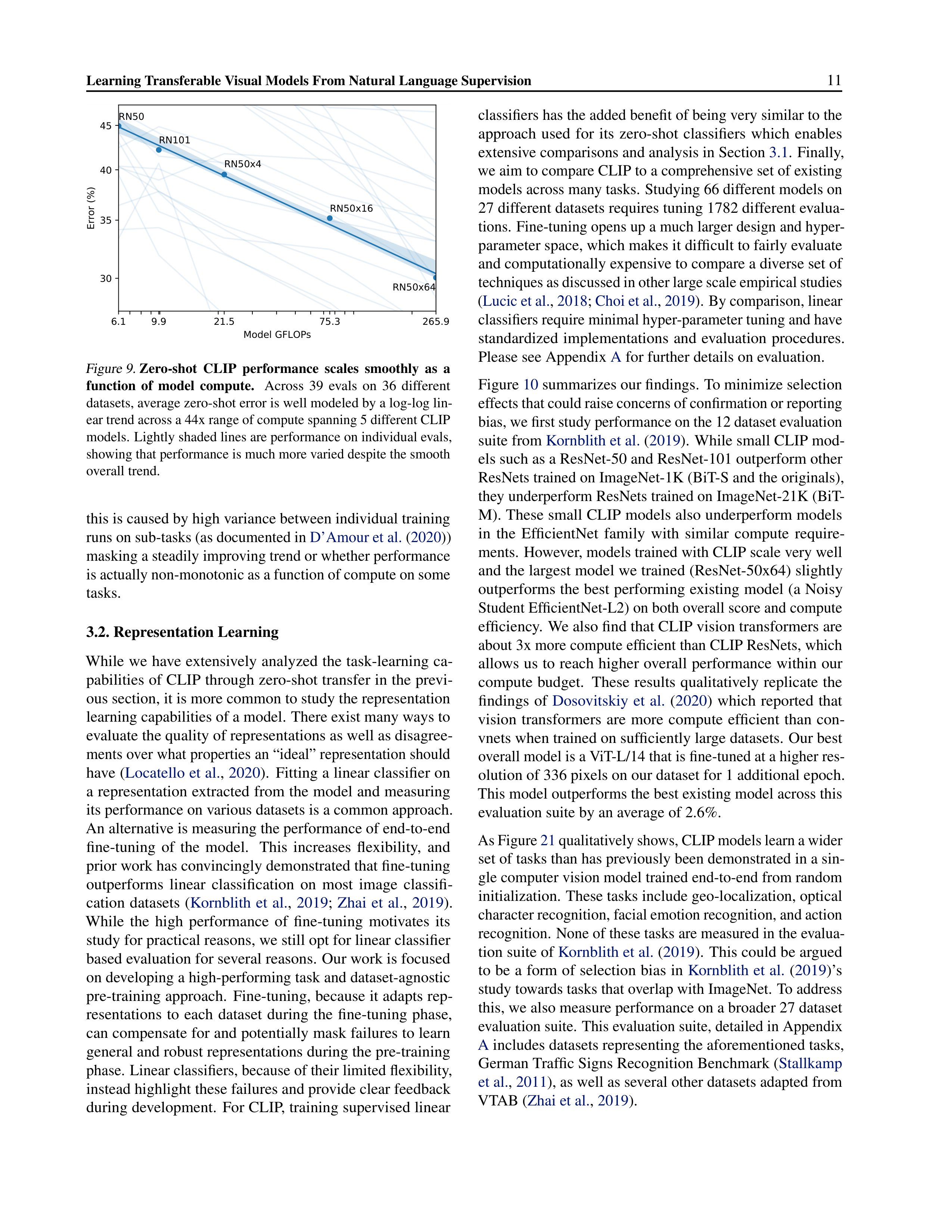
In Figure
9
, we check whether
the zero-shot performance of CLIP follows a similar scaling
pattern.
We plot the average error rate of the 5 ResNet CLIP
models across 39 evaluations on 36 different datasets and
find that a similar log-log linear scaling trend holds for CLIP
across a 44x increase in model compute.
While the overall
trend is smooth, we found that performance on individual
evaluations
can
be
much
noisier.
We
are
unsure
whether
Learning Transferable Visual Models From Natural Language Supervision
11
6.1
9.9
21.5
75.3
265.9
Model GFLOPs
30
35
40
45
Error (%)
RN50
RN101
RN50x4
RN50x16
RN50x64
Figure 9.
Zero-shot
CLIP
performance
scales
smoothly
as
a
function
of
model
compute.
Across
39
evals
on
36
different
datasets, average zero-shot error is well modeled by a log-log lin-
ear trend across a 44x range of compute spanning 5 different CLIP
models.
Lightly shaded lines are performance on individual evals,
showing that performance is much more varied despite the smooth
overall trend.
this is caused by high variance between individual training
runs on sub-tasks (as documented in
D’Amour et al.
(
2020
))
masking a steadily improving trend or whether performance
is actually non-monotonic as a function of compute on some
tasks.
3.2. Representation Learning
While we have extensively analyzed the task-learning ca-
pabilities of CLIP through zero-shot transfer in the previ-
ous section, it is more common to study the representation
learning capabilities of a model.
There exist many ways to
evaluate the quality of representations as well as disagree-
ments over what properties an “ideal” representation should
have (
Locatello et al.
,
2020
).
Fitting a linear classifier on
a representation extracted from the model and measuring
its performance on various datasets is a common approach.
An alternative is measuring the performance of end-to-end
fine-tuning
of
the
model.
This
increases
flexibility,
and
prior work has convincingly demonstrated that fine-tuning
outperforms
linear
classification
on
most
image
classifi-
cation
datasets
(
Kornblith
et
al.
,
2019
;
Zhai
et
al.
,
2019
).
While
the
high
performance
of
fine-tuning
motivates
its
study for practical reasons, we still opt for linear classifier
based evaluation for several reasons.
Our work is focused
on developing a high-performing task and dataset-agnostic
pre-training approach.
Fine-tuning, because it adapts rep-
resentations
to
each
dataset
during
the
fine-tuning
phase,
can compensate for and potentially mask failures to learn
general and robust representations during the pre-training
phase.
Linear classifiers, because of their limited flexibility,
instead highlight these failures and provide clear feedback
during development.
For CLIP, training supervised linear
classifiers has the added benefit of being very similar to the
approach
used
for
its
zero-shot
classifiers
which
enables
extensive comparisons and analysis in Section
3.1
.
Finally,
we aim to compare CLIP to a comprehensive set of existing
models across many tasks.
Studying 66 different models on
27 different datasets requires tuning 1782 different evalua-
tions.
Fine-tuning opens up a much larger design and hyper-
parameter space, which makes it difficult to fairly evaluate
and computationally expensive to compare a diverse set of
techniques as discussed in other large scale empirical studies
(
Lucic et al.
,
2018
;
Choi et al.
,
2019
).
By comparison, linear
classifiers require minimal hyper-parameter tuning and have
standardized
implementations
and
evaluation
procedures.
Please see Appendix
A
for further details on evaluation.
Figure
10
summarizes our findings.
To minimize selection
effects that could raise concerns of confirmation or reporting
bias, we first study performance on the 12 dataset evaluation
suite from
Kornblith et al.
(
2019
).
While small CLIP mod-
els such as a ResNet-50 and ResNet-101 outperform other
ResNets trained on ImageNet-1K (BiT-S and the originals),
they underperform ResNets trained on ImageNet-21K (BiT-
M). These small CLIP models also underperform models
in
the
EfficientNet
family
with
similar
compute
require-
ments.
However, models trained with CLIP scale very well
and the largest model we trained (ResNet-50x64) slightly
outperforms the best performing existing model (a Noisy
Student EfficientNet-L2) on both overall score and compute
efficiency.
We also find that CLIP vision transformers are
about 3x more compute efficient than CLIP ResNets, which
allows
us
to reach
higher
overall
performance within
our
compute
budget.
These
results
qualitatively
replicate
the
findings
of
Dosovitskiy
et
al.
(
2020
)
which
reported
that
vision
transformers
are
more
compute
efficient
than
con-
vnets when trained on sufficiently large datasets.
Our best
overall model is a ViT-L/14 that is fine-tuned at a higher res-
olution of 336 pixels on our dataset for 1 additional epoch.
This model outperforms the best existing model across this
evaluation suite by an average of 2.6%.
As Figure
21
qualitatively shows, CLIP models learn a wider
set of tasks than has previously been demonstrated in a sin-
gle computer vision model trained end-to-end from random
initialization.
These tasks include geo-localization, optical
character recognition, facial emotion recognition, and action
recognition.
None of these tasks are measured in the evalua-
tion suite of
Kornblith et al.
(
2019
).
This could be argued
to be a form of selection bias in
Kornblith et al.
(
2019
)’s
study towards tasks that overlap with ImageNet.
To address
this, we also measure performance on a broader 27 dataset
evaluation suite.
This evaluation suite, detailed in Appendix
A
includes datasets representing the aforementioned tasks,
German Traffic Signs Recognition Benchmark (
Stallkamp
et al.
,
2011
), as well as several other datasets adapted from
VTAB (
Zhai et al.
,
2019
).
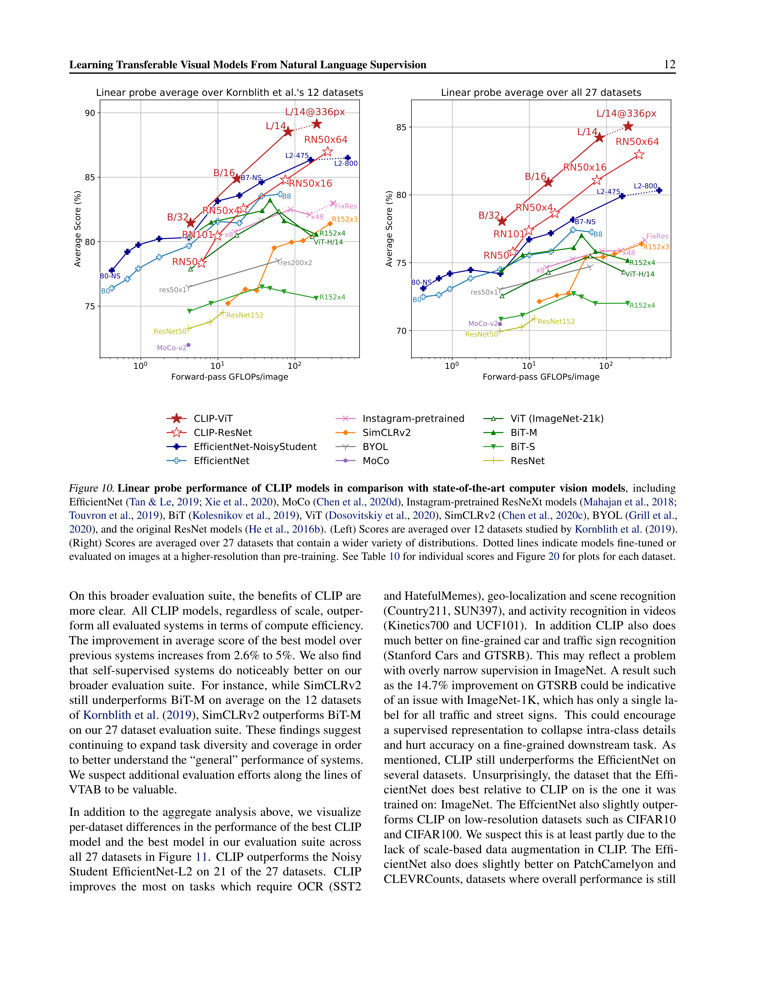
Learning Transferable Visual Models From Natural Language Supervision
12
10
0
10
1
10
2
Forward-pass GFLOPs/image
75
80
85
90
Average Score (%)
Linear probe average over Kornblith et al.'s 12 datasets
10
0
10
1
10
2
Forward-pass GFLOPs/image
70
75
80
85
Average Score (%)
Linear probe average over all 27 datasets
CLIP-ViT
CLIP-ResNet
EfficientNet-NoisyStudent
EfficientNet
Instagram-pretrained
SimCLRv2
BYOL
MoCo
ViT (ImageNet-21k)
BiT-M
BiT-S
ResNet
Figure 10.
Linear
probe
performance
of
CLIP
models
in
comparison
with
state-of-the-art
computer
vision
models
,
including
EfficientNet (
Tan & Le
,
2019
;
Xie et al.
,
2020
), MoCo (
Chen et al.
,
2020d
), Instagram-pretrained ResNeXt models (
Mahajan et al.
,
2018
;
Touvron et al.
,
2019
), BiT (
Kolesnikov et al.
,
2019
), ViT (
Dosovitskiy et al.
,
2020
), SimCLRv2 (
Chen et al.
,
2020c
), BYOL (
Grill et al.
,
2020
), and the original ResNet models (
He et al.
,
2016b
).
(Left) Scores are averaged over 12 datasets studied by
Kornblith et al.
(
2019
).
(Right) Scores are averaged over 27 datasets that contain a wider variety of distributions.
Dotted lines indicate models fine-tuned or
evaluated on images at a higher-resolution than pre-training.
See Table
10
for individual scores and Figure
20
for plots for each dataset.
On this broader evaluation suite, the benefits of CLIP are
more clear.
All CLIP models, regardless of scale, outper-
form all evaluated systems in terms of compute efficiency.
The improvement in average score of the best model over
previous systems increases from 2.6% to 5%.
We also find
that
self-supervised
systems
do
noticeably
better
on
our
broader
evaluation
suite.
For
instance,
while
SimCLRv2
still
underperforms
BiT-M
on
average
on
the
12
datasets
of
Kornblith et al.
(
2019
), SimCLRv2 outperforms BiT-M
on our 27 dataset evaluation suite.
These findings suggest
continuing to expand task diversity and coverage in order
to better understand the “general” performance of systems.
We suspect additional evaluation efforts along the lines of
VTAB to be valuable.
In
addition
to
the
aggregate
analysis
above,
we
visualize
per-dataset differences in the performance of the best CLIP
model
and
the
best
model
in
our
evaluation
suite
across
all 27 datasets in Figure
11
.
CLIP outperforms the Noisy
Student
EfficientNet-L2
on
21
of
the
27
datasets.
CLIP
improves
the
most
on
tasks
which
require
OCR
(SST2
and HatefulMemes), geo-localization and scene recognition
(Country211, SUN397), and activity recognition in videos
(Kinetics700
and
UCF101).
In
addition
CLIP
also
does
much better on fine-grained car and traffic sign recognition
(Stanford
Cars
and
GTSRB).
This
may
reflect
a
problem
with overly narrow supervision in ImageNet.
A result such
as the 14.7% improvement on GTSRB could be indicative
of an issue with ImageNet-1K, which has only a single la-
bel
for
all
traffic
and
street
signs.
This
could
encourage
a
supervised
representation
to
collapse
intra-class
details
and hurt accuracy on a fine-grained downstream task.
As
mentioned,
CLIP
still
underperforms
the
EfficientNet
on
several
datasets.
Unsurprisingly,
the
dataset
that
the
Effi-
cientNet
does
best
relative
to
CLIP
on
is
the
one
it
was
trained on:
ImageNet.
The EffcientNet also slightly outper-
forms CLIP on low-resolution datasets such as CIFAR10
and CIFAR100.
We suspect this is at least partly due to the
lack
of
scale-based
data
augmentation
in
CLIP.
The
Effi-
cientNet
also
does
slightly
better
on
PatchCamelyon
and
CLEVRCounts, datasets where overall performance is still
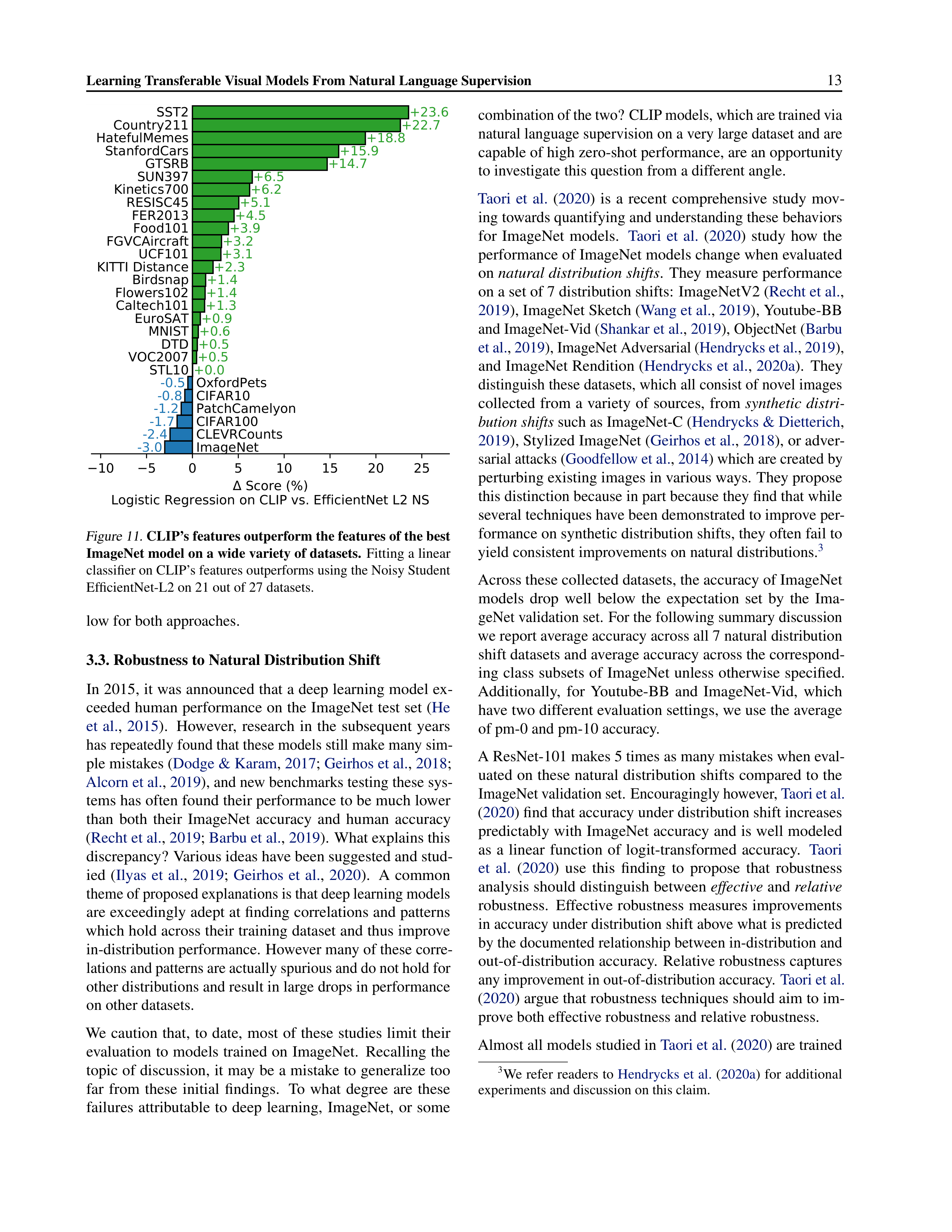
Learning Transferable Visual Models From Natural Language Supervision
13
10
5
0
5
10
15
20
25
Score (%)
Logistic Regression on CLIP vs. EfficientNet L2 NS
ImageNet
-3.0
CLEVRCounts
-2.4
CIFAR100
-1.7
PatchCamelyon
-1.2
CIFAR10
-0.8
OxfordPets
-0.5
+0.0
STL10
+0.5
VOC2007
+0.5
DTD
+0.6
MNIST
+0.9
EuroSAT
+1.3
Caltech101
+1.4
Flowers102
+1.4
Birdsnap
+2.3
KITTI Distance
+3.1
UCF101
+3.2
FGVCAircraft
+3.9
Food101
+4.5
FER2013
+5.1
RESISC45
+6.2
Kinetics700
+6.5
SUN397
+14.7
GTSRB
+15.9
StanfordCars
+18.8
HatefulMemes
+22.7
Country211
+23.6
SST2
Figure 11.
CLIP’s features outperform the features of the best
ImageNet model on a wide variety of datasets.
Fitting a linear
classifier on CLIP’s features outperforms using the Noisy Student
EfficientNet-L2 on 21 out of 27 datasets.
low for both approaches.
3.3. Robustness to Natural Distribution Shift
In 2015, it was announced that a deep learning model ex-
ceeded human performance on the ImageNet test set (
He
et
al.
,
2015
).
However,
research
in
the
subsequent
years
has repeatedly found that these models still make many sim-
ple mistakes (
Dodge & Karam
,
2017
;
Geirhos et al.
,
2018
;
Alcorn et al.
,
2019
), and new benchmarks testing these sys-
tems has often found their performance to be much lower
than
both
their
ImageNet
accuracy
and
human
accuracy
(
Recht et al.
,
2019
;
Barbu et al.
,
2019
).
What explains this
discrepancy?
Various ideas have been suggested and stud-
ied
(
Ilyas
et
al.
,
2019
;
Geirhos
et
al.
,
2020
).
A
common
theme of proposed explanations is that deep learning models
are exceedingly adept at finding correlations and patterns
which hold across their training dataset and thus improve
in-distribution performance.
However many of these corre-
lations and patterns are actually spurious and do not hold for
other distributions and result in large drops in performance
on other datasets.
We
caution
that,
to
date,
most
of
these
studies
limit
their
evaluation to models trained on ImageNet.
Recalling the
topic of discussion, it may be a mistake to generalize too
far
from
these
initial
findings.
To
what
degree
are
these
failures
attributable
to
deep
learning,
ImageNet,
or
some
combination of the two? CLIP models, which are trained via
natural language supervision on a very large dataset and are
capable of high zero-shot performance, are an opportunity
to investigate this question from a different angle.
Taori
et
al.
(
2020
)
is
a
recent
comprehensive
study
mov-
ing towards quantifying and understanding these behaviors
for
ImageNet
models.
Taori
et
al.
(
2020
)
study
how
the
performance of ImageNet models change when evaluated
on
natural distribution shifts
.
They measure performance
on a set of 7 distribution shifts:
ImageNetV2 (
Recht et al.
,
2019
), ImageNet Sketch (
Wang et al.
,
2019
), Youtube-BB
and ImageNet-Vid (
Shankar et al.
,
2019
), ObjectNet (
Barbu
et al.
,
2019
), ImageNet Adversarial (
Hendrycks et al.
,
2019
),
and ImageNet Rendition (
Hendrycks et al.
,
2020a
).
They
distinguish these datasets, which all consist of novel images
collected
from
a
variety
of
sources,
from
synthetic
distri-
bution shifts
such as ImageNet-C (
Hendrycks & Dietterich
,
2019
), Stylized ImageNet (
Geirhos et al.
,
2018
), or adver-
sarial attacks (
Goodfellow et al.
,
2014
) which are created by
perturbing existing images in various ways.
They propose
this distinction because in part because they find that while
several techniques have been demonstrated to improve per-
formance on synthetic distribution shifts, they often fail to
yield consistent improvements on natural distributions.
3
Across these collected datasets, the accuracy of ImageNet
models
drop
well
below
the
expectation
set
by
the
Ima-
geNet validation set.
For the following summary discussion
we report average accuracy across all 7 natural distribution
shift datasets and average accuracy across the correspond-
ing
class
subsets
of
ImageNet
unless
otherwise
specified.
Additionally,
for
Youtube-BB
and
ImageNet-Vid,
which
have two different evaluation settings, we use the average
of pm-0 and pm-10 accuracy.
A ResNet-101 makes 5 times as many mistakes when eval-
uated on these natural distribution shifts compared to the
ImageNet validation set.
Encouragingly however,
Taori et al.
(
2020
) find that accuracy under distribution shift increases
predictably with ImageNet accuracy and is well modeled
as
a
linear
function
of
logit-transformed
accuracy.
Taori
et
al.
(
2020
)
use
this
finding
to
propose
that
robustness
analysis should distinguish between
effective
and
relative
robustness.
Effective
robustness
measures
improvements
in accuracy under distribution shift above what is predicted
by the documented relationship between in-distribution and
out-of-distribution accuracy.
Relative robustness captures
any improvement in out-of-distribution accuracy.
Taori et al.
(
2020
) argue that robustness techniques should aim to im-
prove both effective robustness and relative robustness.
Almost all models studied in
Taori et al.
(
2020
) are trained
3
We refer readers to
Hendrycks et al.
(
2020a
) for additional
experiments and discussion on this claim.
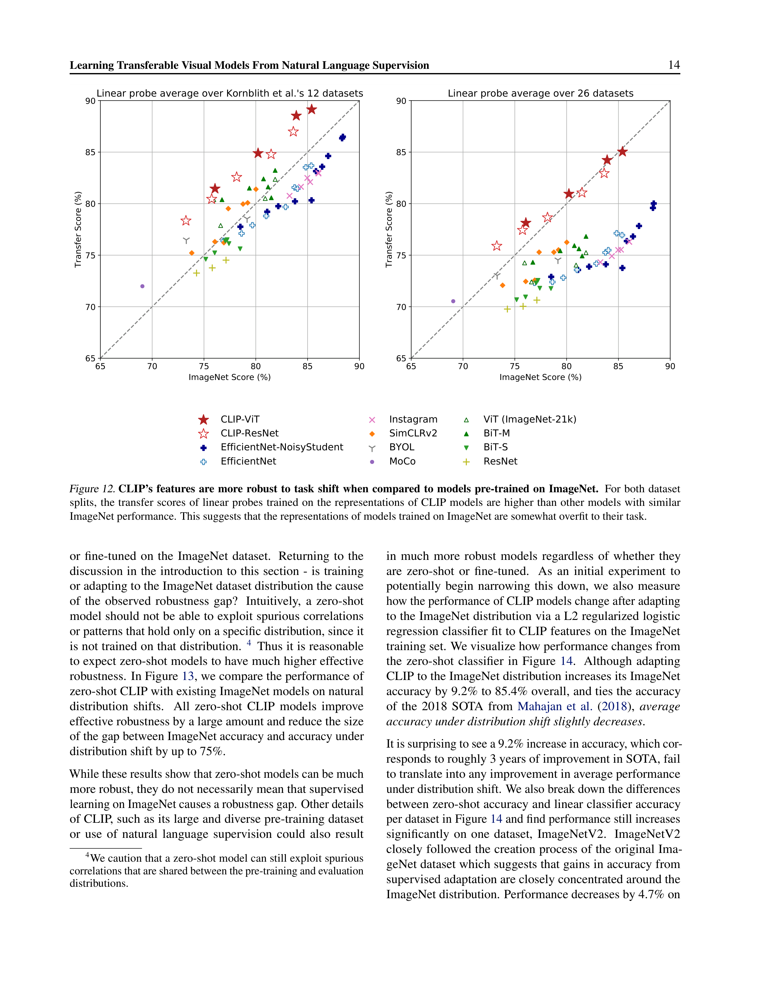
Learning Transferable Visual Models From Natural Language Supervision
14
65
70
75
80
85
90
ImageNet Score (%)
65
70
75
80
85
90
Transfer Score (%)
Linear probe average over Kornblith et al.'s 12 datasets
65
70
75
80
85
90
ImageNet Score (%)
65
70
75
80
85
90
Transfer Score (%)
Linear probe average over 26 datasets
CLIP-ViT
CLIP-ResNet
EfficientNet-NoisyStudent
EfficientNet
Instagram
SimCLRv2
BYOL
MoCo
ViT (ImageNet-21k)
BiT-M
BiT-S
ResNet
Figure 12.
CLIP’s
features
are
more
robust
to
task
shift
when
compared
to
models
pre-trained
on
ImageNet.
For
both
dataset
splits,
the
transfer
scores
of
linear
probes
trained
on
the
representations
of
CLIP
models
are
higher
than
other
models
with
similar
ImageNet performance.
This suggests that the representations of models trained on ImageNet are somewhat overfit to their task.
or
fine-tuned
on
the
ImageNet
dataset.
Returning
to
the
discussion
in
the
introduction
to
this
section
-
is
training
or adapting to the ImageNet dataset distribution the cause
of
the
observed
robustness
gap?
Intuitively,
a
zero-shot
model should not be able to exploit spurious correlations
or patterns that hold only on a specific distribution, since it
is not trained on that distribution.
4
Thus it is reasonable
to expect zero-shot models to have much higher effective
robustness.
In Figure
13
, we compare the performance of
zero-shot CLIP with existing ImageNet models on natural
distribution
shifts.
All
zero-shot
CLIP
models
improve
effective robustness by a large amount and reduce the size
of the gap between ImageNet accuracy and accuracy under
distribution shift by up to 75%.
While these results show that zero-shot models can be much
more robust, they do not necessarily mean that supervised
learning on ImageNet causes a robustness gap.
Other details
of CLIP, such as its large and diverse pre-training dataset
or
use
of
natural
language
supervision
could
also
result
4
We caution that a zero-shot model can still exploit spurious
correlations that are shared between the pre-training and evaluation
distributions.
in
much
more
robust
models
regardless
of
whether
they
are
zero-shot
or
fine-tuned.
As
an
initial
experiment
to
potentially
begin
narrowing
this
down,
we
also
measure
how the performance of CLIP models change after adapting
to the ImageNet distribution via a L2 regularized logistic
regression classifier fit to CLIP features on the ImageNet
training set.
We visualize how performance changes from
the
zero-shot
classifier
in
Figure
14
.
Although
adapting
CLIP to the ImageNet distribution increases its ImageNet
accuracy by 9.2% to 85.4% overall, and ties the accuracy
of
the
2018
SOTA
from
Mahajan
et
al.
(
2018
),
average
accuracy under distribution shift slightly decreases
.
It is surprising to see a 9.2% increase in accuracy, which cor-
responds to roughly 3 years of improvement in SOTA, fail
to translate into any improvement in average performance
under distribution shift.
We also break down the differences
between zero-shot accuracy and linear classifier accuracy
per dataset in Figure
14
and find performance still increases
significantly
on
one
dataset,
ImageNetV2.
ImageNetV2
closely followed the creation process of the original Ima-
geNet dataset which suggests that gains in accuracy from
supervised adaptation are closely concentrated around the
ImageNet distribution.
Performance decreases by 4.7% on
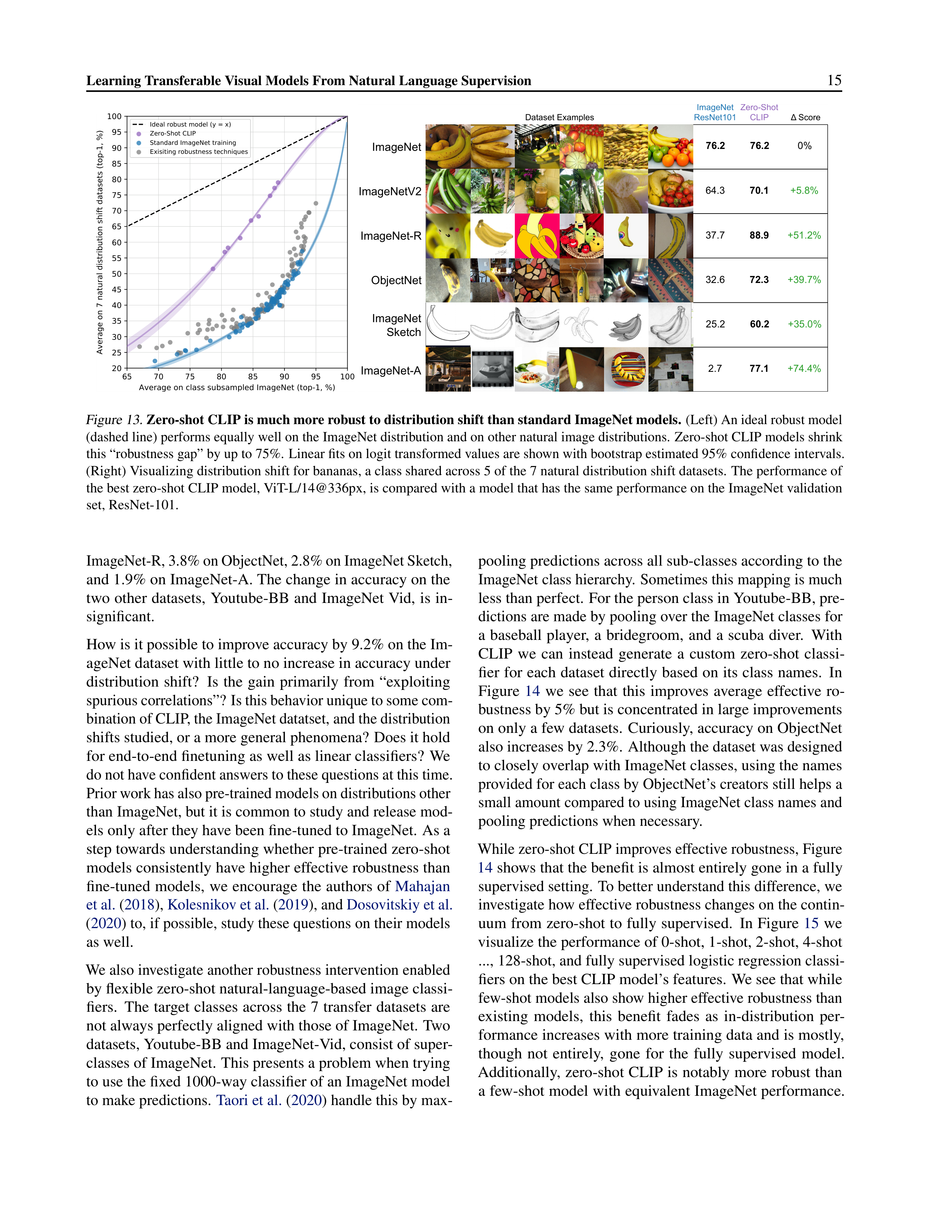
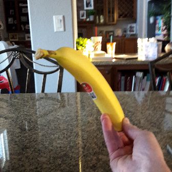




Learning Transferable Visual Models From Natural Language Supervision
15
65
70
75
80
85
90
95
100
Average on class subsampled ImageNet (top-1, %)
20
25
30
35
40
45
50
55
60
65
70
75
80
85
90
95
100
Average on 7 natural distribution shift datasets (top-1, %)
Ideal robust model (y = x)
Zero-Shot CLIP
Standard ImageNet training
Exisiting robustness techniques
ImageNet
ImageNetV2
ImageNet-A
ImageNet-R
ObjectNet
ImageNet
Sketch
76.2
76.2
64.3
70.1
2.7
77.1
37.7
88.9
32.6
72.3
25.2
60.2
ImageNet
ResNet101
Zero-Shot
CLIP
0%
+5.8%
+74.4%
+51.2%
+39.7%
+35.0%
Δ Score
Dataset Examples
Figure 13.
Zero-shot CLIP is much more robust to distribution shift than standard ImageNet models.
(Left) An ideal robust model
(dashed line) performs equally well on the ImageNet distribution and on other natural image distributions.
Zero-shot CLIP models shrink
this “robustness gap” by up to 75%.
Linear fits on logit transformed values are shown with bootstrap estimated 95% confidence intervals.
(Right) Visualizing distribution shift for bananas, a class shared across 5 of the 7 natural distribution shift datasets.
The performance of
the best zero-shot CLIP model, ViT-L/14@336px, is compared with a model that has the same performance on the ImageNet validation
set, ResNet-101.
ImageNet-R, 3.8% on ObjectNet, 2.8% on ImageNet Sketch,
and 1.9% on ImageNet-A. The change in accuracy on the
two other datasets,
Youtube-BB and ImageNet Vid,
is in-
significant.
How is it possible to improve accuracy by 9.2% on the Im-
ageNet dataset with little to no increase in accuracy under
distribution
shift?
Is
the
gain
primarily
from
“exploiting
spurious correlations”? Is this behavior unique to some com-
bination of CLIP, the ImageNet datatset, and the distribution
shifts studied, or a more general phenomena?
Does it hold
for end-to-end finetuning as well as linear classifiers?
We
do not have confident answers to these questions at this time.
Prior work has also pre-trained models on distributions other
than ImageNet, but it is common to study and release mod-
els only after they have been fine-tuned to ImageNet.
As a
step towards understanding whether pre-trained zero-shot
models consistently have higher effective robustness than
fine-tuned models,
we encourage the authors of
Mahajan
et al.
(
2018
),
Kolesnikov et al.
(
2019
), and
Dosovitskiy et al.
(
2020
) to, if possible, study these questions on their models
as well.
We also investigate another robustness intervention enabled
by flexible zero-shot natural-language-based image classi-
fiers.
The target classes across the 7 transfer datasets are
not always perfectly aligned with those of ImageNet.
Two
datasets, Youtube-BB and ImageNet-Vid, consist of super-
classes of ImageNet.
This presents a problem when trying
to use the fixed 1000-way classifier of an ImageNet model
to make predictions.
Taori et al.
(
2020
) handle this by max-
pooling predictions across all sub-classes according to the
ImageNet class hierarchy.
Sometimes this mapping is much
less than perfect.
For the person class in Youtube-BB, pre-
dictions are made by pooling over the ImageNet classes for
a
baseball
player,
a
bridegroom,
and
a
scuba
diver.
With
CLIP
we
can
instead
generate
a
custom
zero-shot
classi-
fier for each dataset directly based on its class names.
In
Figure
14
we
see
that
this
improves
average
effective
ro-
bustness by 5% but is concentrated in large improvements
on only a few datasets.
Curiously, accuracy on ObjectNet
also increases by 2.3%.
Although the dataset was designed
to closely overlap with ImageNet classes, using the names
provided for each class by ObjectNet’s creators still helps a
small amount compared to using ImageNet class names and
pooling predictions when necessary.
While zero-shot CLIP improves effective robustness, Figure
14
shows that the benefit is almost entirely gone in a fully
supervised setting.
To better understand this difference, we
investigate how effective robustness changes on the contin-
uum from zero-shot to fully supervised.
In Figure
15
we
visualize the performance of 0-shot, 1-shot, 2-shot, 4-shot
..., 128-shot, and fully supervised logistic regression classi-
fiers on the best CLIP model’s features.
We see that while
few-shot models also show higher effective robustness than
existing
models,
this
benefit
fades
as
in-distribution
per-
formance increases with more training data and is mostly,
though
not
entirely,
gone
for
the
fully
supervised
model.
Additionally, zero-shot CLIP is notably more robust than
a few-shot model with equivalent ImageNet performance.
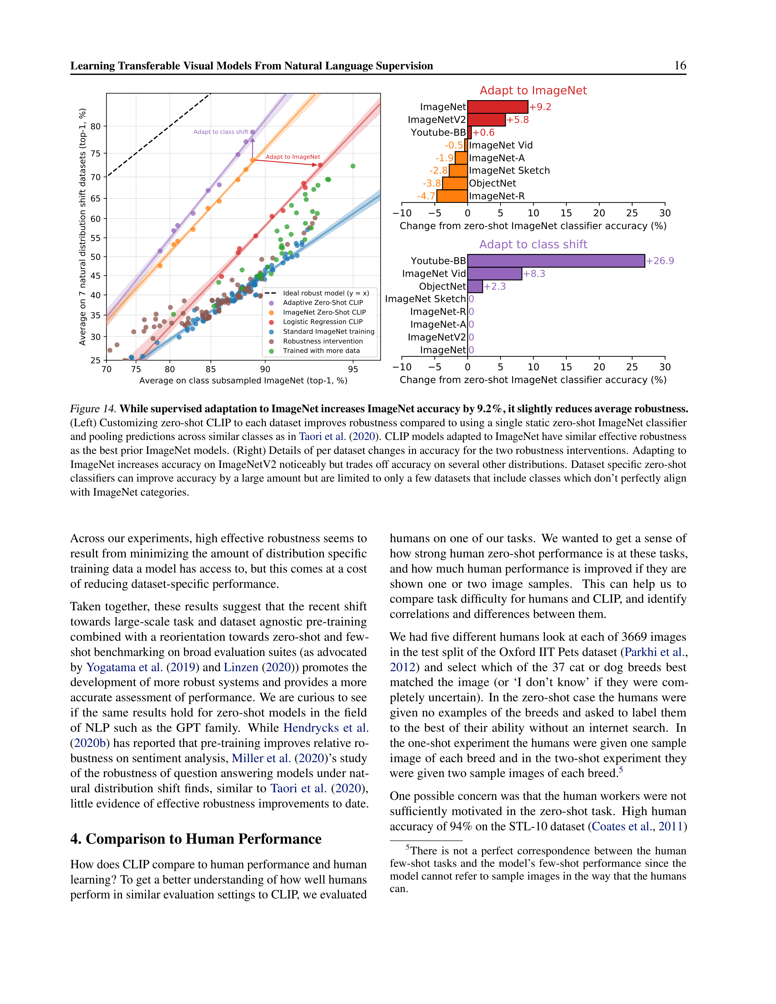
Learning Transferable Visual Models From Natural Language Supervision
16
70
75
80
85
90
95
Average on class subsampled ImageNet (top-1, %)
25
30
35
40
45
50
55
60
65
70
75
80
Average on 7 natural distribution shift datasets (top-1, %)
Adapt to class shift
Adapt to ImageNet
Ideal robust model (y = x)
Adaptive Zero-Shot CLIP
ImageNet Zero-Shot CLIP
Logistic Regression CLIP
Standard ImageNet training
Robustness intervention
Trained with more data
10
5
0
5
10
15
20
25
30
Change from zero-shot ImageNet classifier accuracy (%)
ImageNet-R
-4.7
ObjectNet
-3.8
ImageNet Sketch
-2.8
ImageNet-A
-1.9
ImageNet Vid
-0.5
+0.6
Youtube-BB
+5.8
ImageNetV2
+9.2
ImageNet
Adapt to ImageNet
10
5
0
5
10
15
20
25
30
Change from zero-shot ImageNet classifier accuracy (%)
0
ImageNet
0
ImageNetV2
0
ImageNet-A
0
ImageNet-R
0
ImageNet Sketch
+2.3
ObjectNet
+8.3
ImageNet Vid
+26.9
Youtube-BB
Adapt to class shift
Figure 14.
While supervised adaptation to ImageNet increases ImageNet accuracy by 9.2%, it slightly reduces average robustness.
(Left) Customizing zero-shot CLIP to each dataset improves robustness compared to using a single static zero-shot ImageNet classifier
and pooling predictions across similar classes as in
Taori et al.
(
2020
).
CLIP models adapted to ImageNet have similar effective robustness
as the best prior ImageNet models.
(Right) Details of per dataset changes in accuracy for the two robustness interventions.
Adapting to
ImageNet increases accuracy on ImageNetV2 noticeably but trades off accuracy on several other distributions.
Dataset specific zero-shot
classifiers can improve accuracy by a large amount but are limited to only a few datasets that include classes which don’t perfectly align
with ImageNet categories.
Across our experiments, high effective robustness seems to
result from minimizing the amount of distribution specific
training data a model has access to, but this comes at a cost
of reducing dataset-specific performance.
Taken
together,
these
results
suggest
that
the
recent
shift
towards large-scale task and dataset agnostic pre-training
combined with a reorientation towards zero-shot and few-
shot benchmarking on broad evaluation suites (as advocated
by
Yogatama et al.
(
2019
) and
Linzen
(
2020
)) promotes the
development of more robust systems and provides a more
accurate assessment of performance.
We are curious to see
if
the
same
results
hold
for
zero-shot
models
in
the
field
of
NLP
such
as
the
GPT
family.
While
Hendrycks
et
al.
(
2020b
) has reported that pre-training improves relative ro-
bustness on sentiment analysis,
Miller et al.
(
2020
)’s study
of the robustness of question answering models under nat-
ural
distribution
shift
finds,
similar
to
Taori
et
al.
(
2020
),
little evidence of effective robustness improvements to date.
4. Comparison to Human Performance
How does CLIP compare to human performance and human
learning?
To get a better understanding of how well humans
perform in similar evaluation settings to CLIP, we evaluated
humans on one of our tasks.
We wanted to get a sense of
how strong human zero-shot performance is at these tasks,
and how much human performance is improved if they are
shown
one
or
two
image
samples.
This
can
help
us
to
compare task difficulty for humans and CLIP, and identify
correlations and differences between them.
We had five different humans look at each of 3669 images
in the test split of the Oxford IIT Pets dataset (
Parkhi et al.
,
2012
)
and
select
which
of
the
37
cat
or
dog
breeds
best
matched
the
image
(or
‘I
don’t
know’
if
they
were
com-
pletely uncertain).
In the zero-shot case the humans were
given
no
examples
of
the
breeds
and
asked
to
label
them
to
the
best
of
their
ability
without
an
internet
search.
In
the one-shot experiment the humans were given one sample
image of each breed and in the two-shot experiment they
were given two sample images of each breed.
5
One possible concern was that the human workers were not
sufficiently
motivated
in
the
zero-shot
task.
High
human
accuracy of 94% on the STL-10 dataset (
Coates et al.
,
2011
)
5
There
is
not
a
perfect
correspondence
between
the
human
few-shot
tasks
and
the
model’s
few-shot
performance
since
the
model cannot refer to sample images in the way that the humans
can.
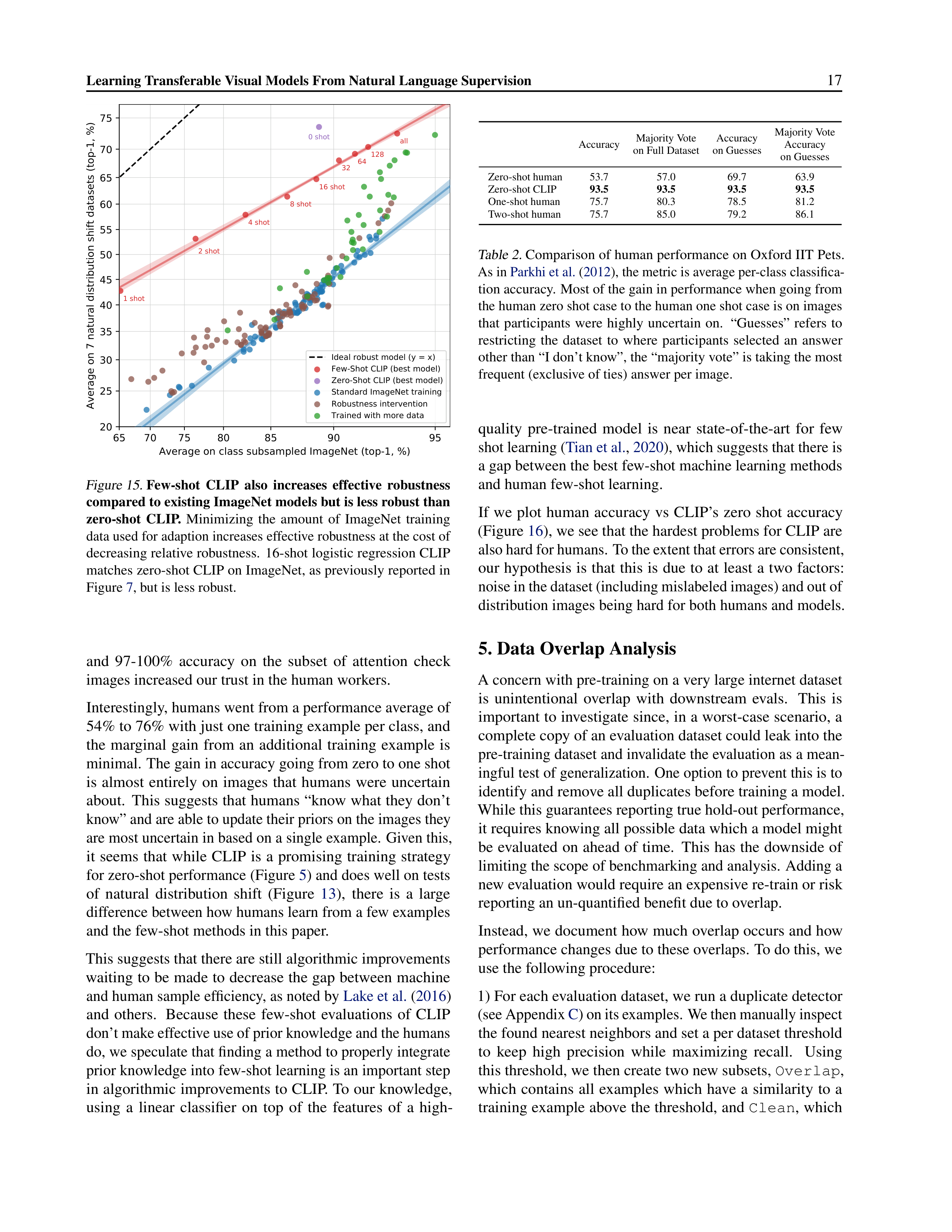
Learning Transferable Visual Models From Natural Language Supervision
17
65
70
75
80
85
90
95
Average on class subsampled ImageNet (top-1, %)
20
25
30
35
40
45
50
55
60
65
70
75
Average on 7 natural distribution shift datasets (top-1, %)
1 shot
2 shot
4 shot
8 shot
16 shot
32
64
128
all
0 shot
Ideal robust model (y = x)
Few-Shot CLIP (best model)
Zero-Shot CLIP (best model)
Standard ImageNet training
Robustness intervention
Trained with more data
Figure 15.
Few-shot
CLIP
also
increases
effective
robustness
compared to existing ImageNet models but is less robust than
zero-shot
CLIP.
Minimizing
the
amount
of
ImageNet
training
data used for adaption increases effective robustness at the cost of
decreasing relative robustness.
16-shot logistic regression CLIP
matches zero-shot CLIP on ImageNet, as previously reported in
Figure
7
, but is less robust.
and
97-100%
accuracy
on
the
subset
of
attention
check
images increased our trust in the human workers.
Interestingly, humans went from a performance average of
54% to 76% with just one training example per class, and
the
marginal
gain
from
an
additional
training
example
is
minimal.
The gain in accuracy going from zero to one shot
is
almost
entirely
on
images
that
humans
were
uncertain
about.
This suggests that humans “know what they don’t
know” and are able to update their priors on the images they
are most uncertain in based on a single example.
Given this,
it
seems
that
while
CLIP
is
a
promising
training
strategy
for zero-shot performance (Figure
5
) and does well on tests
of
natural
distribution
shift
(Figure
13
),
there
is
a
large
difference between how humans learn from a few examples
and the few-shot methods in this paper.
This suggests that there are still algorithmic improvements
waiting to be made to decrease the gap between machine
and human sample efficiency, as noted by
Lake et al.
(
2016
)
and
others.
Because
these
few-shot
evaluations
of
CLIP
don’t make effective use of prior knowledge and the humans
do, we speculate that finding a method to properly integrate
prior knowledge into few-shot learning is an important step
in algorithmic improvements to CLIP. To our knowledge,
using
a
linear
classifier
on
top
of
the
features
of
a
high-
Accuracy
Majority Vote
on Full Dataset
Accuracy
on Guesses
Majority Vote
Accuracy
on Guesses
Zero-shot human
53.7
57.0
69.7
63.9
Zero-shot CLIP
93.5
93.5
93.5
93.5
One-shot human
75.7
80.3
78.5
81.2
Two-shot human
75.7
85.0
79.2
86.1
Table 2.
Comparison of human performance on Oxford IIT Pets.
As in
Parkhi et al.
(
2012
), the metric is average per-class classifica-
tion accuracy.
Most of the gain in performance when going from
the human zero shot case to the human one shot case is on images
that
participants
were
highly
uncertain
on.
“Guesses”
refers
to
restricting
the
dataset
to
where
participants
selected
an
answer
other than “I don’t know”, the “majority vote” is taking the most
frequent (exclusive of ties) answer per image.
quality
pre-trained
model
is
near
state-of-the-art
for
few
shot learning (
Tian et al.
,
2020
), which suggests that there is
a gap between the best few-shot machine learning methods
and human few-shot learning.
If
we
plot
human
accuracy
vs
CLIP’s
zero
shot
accuracy
(Figure
16
), we see that the hardest problems for CLIP are
also hard for humans. To the extent that errors are consistent,
our
hypothesis
is
that
this
is
due
to
at
least
a
two
factors:
noise in the dataset (including mislabeled images) and out of
distribution images being hard for both humans and models.
5. Data Overlap Analysis
A concern with pre-training on a very large internet dataset
is
unintentional
overlap
with
downstream
evals.
This
is
important to investigate since, in a worst-case scenario, a
complete copy of an evaluation dataset could leak into the
pre-training dataset and invalidate the evaluation as a mean-
ingful test of generalization.
One option to prevent this is to
identify and remove all duplicates before training a model.
While this guarantees reporting true hold-out performance,
it requires knowing all possible data which a model might
be evaluated on ahead of time.
This has the downside of
limiting the scope of benchmarking and analysis.
Adding a
new evaluation would require an expensive re-train or risk
reporting an un-quantified benefit due to overlap.
Instead, we document how much overlap occurs and how
performance changes due to these overlaps.
To do this, we
use the following procedure:
1) For each evaluation dataset, we run a duplicate detector
(see Appendix
C
) on its examples. We then manually inspect
the found nearest neighbors and set a per dataset threshold
to
keep
high
precision
while
maximizing
recall.
Using
this threshold, we then create two new subsets,
Overlap
,
which
contains
all
examples
which
have
a
similarity
to
a
training example above the threshold, and
Clean
, which
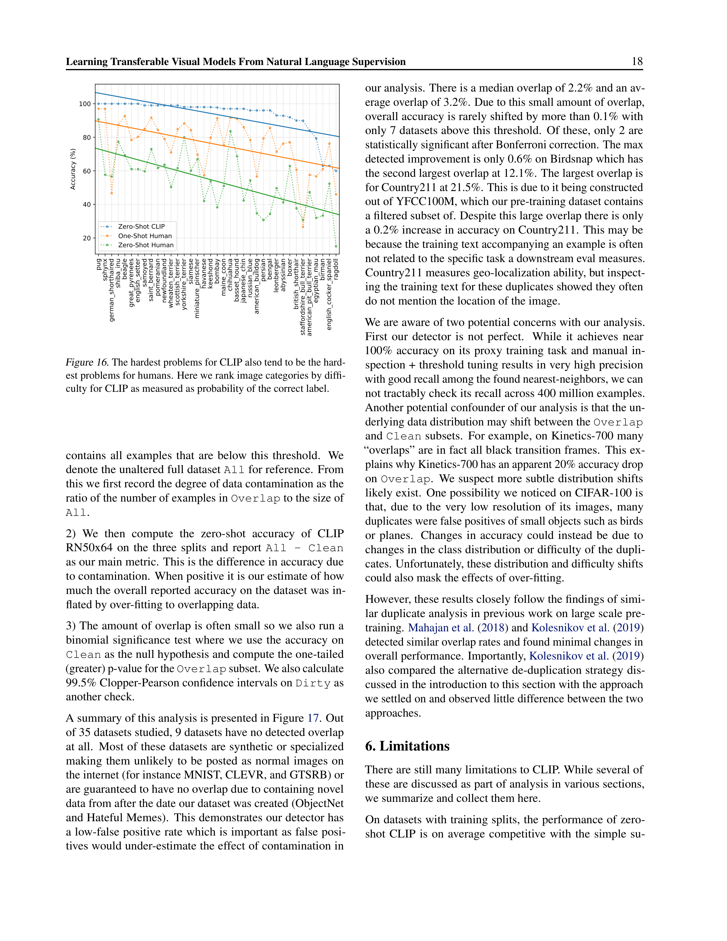
Learning Transferable Visual Models From Natural Language Supervision
18
pug
sphynx
german_shorthaired
shiba_inu
beagle
great_pyrenees
english_setter
samoyed
saint_bernard
pomeranian
newfoundland
wheaten_terrier
scottish_terrier
yorkshire_terrier
siamese
miniature_pinscher
havanese
keeshond
bombay
maine_coon
chihuahua
basset_hound
japanese_chin
russian_blue
american_bulldog
persian
bengal
leonberger
abyssinian
boxer
british_shorthair
staffordshire_bull_terrier
american_pit_bull_terrier
egyptian_mau
birman
english_cocker_spaniel
ragdoll
20
40
60
80
100
Accuracy (%)
Zero-Shot CLIP
One-Shot Human
Zero-Shot Human
Figure 16.
The hardest problems for CLIP also tend to be the hard-
est problems for humans.
Here we rank image categories by diffi-
culty for CLIP as measured as probability of the correct label.
contains
all
examples
that
are
below
this
threshold.
We
denote the unaltered full dataset
All
for reference.
From
this we first record the degree of data contamination as the
ratio of the number of examples in
Overlap
to the size of
All
.
2)
We
then
compute
the
zero-shot
accuracy
of
CLIP
RN50x64
on
the
three
splits
and
report
All
-
Clean
as our main metric.
This is the difference in accuracy due
to contamination.
When positive it is our estimate of how
much the overall reported accuracy on the dataset was in-
flated by over-fitting to overlapping data.
3) The amount of overlap is often small so we also run a
binomial
significance
test
where
we
use
the
accuracy
on
Clean
as the null hypothesis and compute the one-tailed
(greater) p-value for the
Overlap
subset. We also calculate
99.5% Clopper-Pearson confidence intervals on
Dirty
as
another check.
A summary of this analysis is presented in Figure
17
.
Out
of 35 datasets studied, 9 datasets have no detected overlap
at all.
Most of
these datasets are synthetic or specialized
making
them
unlikely
to
be
posted
as
normal
images
on
the internet (for instance MNIST, CLEVR, and GTSRB) or
are guaranteed to have no overlap due to containing novel
data from after the date our dataset was created (ObjectNet
and Hateful Memes).
This demonstrates our detector has
a
low-false
positive
rate
which
is
important
as
false
posi-
tives would under-estimate the effect of contamination in
our analysis.
There is a median overlap of 2.2% and an av-
erage overlap of 3.2%.
Due to this small amount of overlap,
overall accuracy is rarely shifted by more than 0.1% with
only 7 datasets above this threshold.
Of these, only 2 are
statistically significant after Bonferroni correction.
The max
detected improvement is only 0.6% on Birdsnap which has
the second largest overlap at 12.1%.
The largest overlap is
for Country211 at 21.5%.
This is due to it being constructed
out of YFCC100M, which our pre-training dataset contains
a filtered subset of.
Despite this large overlap there is only
a 0.2% increase in accuracy on Country211.
This may be
because the training text accompanying an example is often
not related to the specific task a downstream eval measures.
Country211 measures geo-localization ability, but inspect-
ing the training text for these duplicates showed they often
do not mention the location of the image.
We are aware of two potential concerns with our analysis.
First
our
detector
is
not
perfect.
While
it
achieves
near
100%
accuracy
on
its
proxy
training
task
and
manual
in-
spection + threshold tuning results in very high precision
with good recall among the found nearest-neighbors, we can
not tractably check its recall across 400 million examples.
Another potential confounder of our analysis is that the un-
derlying data distribution may shift between the
Overlap
and
Clean
subsets.
For example,
on Kinetics-700 many
“overlaps” are in fact all black transition frames.
This ex-
plains why Kinetics-700 has an apparent 20% accuracy drop
on
Overlap
.
We suspect more subtle distribution shifts
likely exist.
One possibility we noticed on CIFAR-100 is
that,
due
to
the
very
low
resolution
of
its
images,
many
duplicates were false positives of small objects such as birds
or
planes.
Changes
in
accuracy
could
instead
be
due
to
changes in the class distribution or difficulty of the dupli-
cates.
Unfortunately, these distribution and difficulty shifts
could also mask the effects of over-fitting.
However, these results closely follow the findings of simi-
lar duplicate analysis in previous work on large scale pre-
training.
Mahajan et al.
(
2018
) and
Kolesnikov et al.
(
2019
)
detected similar overlap rates and found minimal changes in
overall performance.
Importantly,
Kolesnikov et al.
(
2019
)
also
compared
the
alternative
de-duplication
strategy
dis-
cussed in the introduction to this section with the approach
we settled on and observed little difference between the two
approaches.
6. Limitations
There are still many limitations to CLIP. While several of
these are discussed as part of analysis in various sections,
we summarize and collect them here.
On datasets with training splits,
the performance of zero-
shot
CLIP
is
on
average
competitive
with
the
simple
su-
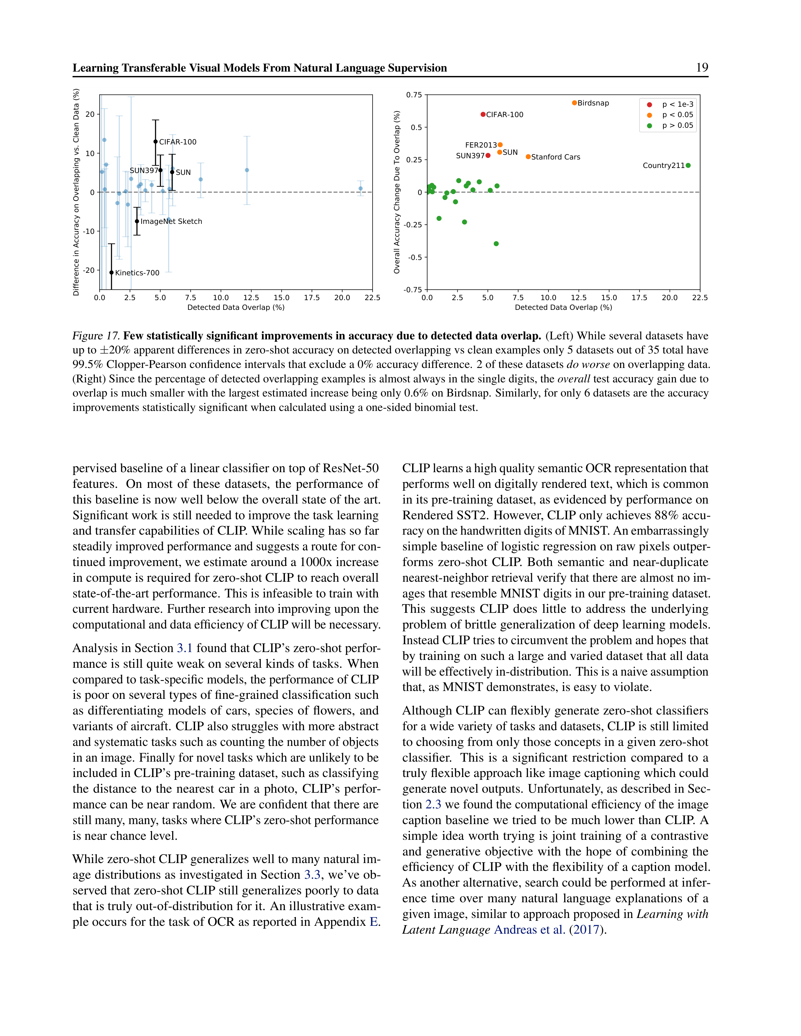
Learning Transferable Visual Models From Natural Language Supervision
19
0.0
2.5
5.0
7.5
10.0
12.5
15.0
17.5
20.0
22.5
Detected Data Overlap (%)
-20
-10
0
10
20
Difference in Accuracy on Overlapping vs. Clean Data (%)
SUN397
CIFAR-100
ImageNet Sketch
SUN
Kinetics-700
0.0
2.5
5.0
7.5
10.0
12.5
15.0
17.5
20.0
22.5
Detected Data Overlap (%)
-0.75
-0.5
-0.25
0
0.25
0.5
0.75
Overall Accuracy Change Due To Overlap (%)
Stanford Cars
SUN397
Birdsnap
CIFAR-100
FER2013
Country211
SUN
p < 1e-3
p < 0.05
p > 0.05
Figure 17.
Few statistically significant improvements in accuracy due to detected data overlap.
(Left) While several datasets have
up to
±
20% apparent differences in zero-shot accuracy on detected overlapping vs clean examples only 5 datasets out of 35 total have
99.5% Clopper-Pearson confidence intervals that exclude a 0% accuracy difference.
2 of these datasets
do worse
on overlapping data.
(Right) Since the percentage of detected overlapping examples is almost always in the single digits, the
overall
test accuracy gain due to
overlap is much smaller with the largest estimated increase being only 0.6% on Birdsnap.
Similarly, for only 6 datasets are the accuracy
improvements statistically significant when calculated using a one-sided binomial test.
pervised baseline of a linear classifier on top of ResNet-50
features.
On
most
of
these
datasets,
the
performance
of
this baseline is now well below the overall state of the art.
Significant work is still needed to improve the task learning
and transfer capabilities of CLIP. While scaling has so far
steadily improved performance and suggests a route for con-
tinued improvement, we estimate around a 1000x increase
in compute is required for zero-shot CLIP to reach overall
state-of-the-art performance.
This is infeasible to train with
current hardware.
Further research into improving upon the
computational and data efficiency of CLIP will be necessary.
Analysis in Section
3.1
found that CLIP’s zero-shot perfor-
mance is still quite weak on several kinds of tasks.
When
compared to task-specific models, the performance of CLIP
is poor on several types of fine-grained classification such
as
differentiating
models
of
cars,
species
of
flowers,
and
variants of aircraft.
CLIP also struggles with more abstract
and systematic tasks such as counting the number of objects
in an image.
Finally for novel tasks which are unlikely to be
included in CLIP’s pre-training dataset, such as classifying
the
distance
to
the
nearest
car
in
a
photo,
CLIP’s
perfor-
mance can be near random.
We are confident that there are
still many, many, tasks where CLIP’s zero-shot performance
is near chance level.
While zero-shot CLIP generalizes well to many natural im-
age distributions as investigated in Section
3.3
, we’ve ob-
served that zero-shot CLIP still generalizes poorly to data
that is truly out-of-distribution for it.
An illustrative exam-
ple occurs for the task of OCR as reported in Appendix
E
.
CLIP learns a high quality semantic OCR representation that
performs well on digitally rendered text, which is common
in its pre-training dataset, as evidenced by performance on
Rendered SST2.
However, CLIP only achieves 88% accu-
racy on the handwritten digits of MNIST. An embarrassingly
simple baseline of logistic regression on raw pixels outper-
forms
zero-shot
CLIP.
Both
semantic
and
near-duplicate
nearest-neighbor retrieval verify that there are almost no im-
ages that resemble MNIST digits in our pre-training dataset.
This
suggests
CLIP
does
little
to
address
the
underlying
problem of brittle generalization of deep learning models.
Instead CLIP tries to circumvent the problem and hopes that
by training on such a large and varied dataset that all data
will be effectively in-distribution. This is a naive assumption
that, as MNIST demonstrates, is easy to violate.
Although CLIP can flexibly generate zero-shot classifiers
for a wide variety of tasks and datasets, CLIP is still limited
to choosing from only those concepts in a given zero-shot
classifier.
This
is
a
significant
restriction
compared
to
a
truly flexible approach like image captioning which could
generate novel outputs.
Unfortunately, as described in Sec-
tion
2.3
we found the computational efficiency of the image
caption baseline we tried to be much lower than CLIP. A
simple
idea
worth
trying
is
joint
training
of
a
contrastive
and
generative
objective
with
the
hope
of
combining
the
efficiency of CLIP with the flexibility of a caption model.
As another alternative, search could be performed at infer-
ence
time
over
many
natural
language
explanations
of
a
given image, similar to approach proposed in
Learning with
Latent Language
Andreas et al.
(
2017
).
Learning Transferable Visual Models From Natural Language Supervision
20
CLIP also does not address the poor data efficiency of deep
learning.
Instead CLIP compensates by using a source of
supervision
that
can
be
scaled
to
hundreds
of
millions
of
training examples.
If every image seen during training of
a
CLIP
model
was
presented
at
a
rate
of
one
per
second,
it would take 405 years to iterate through the 12.8 billion
images
seen
over
32
training
epochs.
Combining
CLIP
with self-supervision (
Henaff
,
2020
;
Chen et al.
,
2020c
) and
self-training (
Lee
;
Xie et al.
,
2020
) methods is a promising
direction given their demonstrated ability to improve data
efficiency over standard supervised learning.
Our
methodology
has
several
significant
limitations.
De-
spite our focus on zero-shot transfer, we repeatedly queried
performance
on
full
validation
sets
to
guide
the
develop-
ment of CLIP. These validation sets often have thousands
of
examples,
which
is
unrealistic
for
true
zero-shot
sce-
narios.
Similar
concerns
have
been
raised
in
the
field
of
semi-supervised learning (
Oliver et al.
,
2018
).
Another po-
tential issue is our selection of evaluation datasets.
While
we
have
reported
results
on
Kornblith
et
al.
(
2019
)’s
12
dataset
evaluation
suite
as
a
standardized
collection,
our
main
results
use
a
somewhat
haphazardly
assembled
col-
lection
of
27
datasets
that
is
undeniably
co-adapted
with
the development and capabilities of CLIP. Creating a new
benchmark
of
tasks
designed
explicitly
to
evaluate
broad
zero-shot transfer capabilities, rather than re-using existing
supervised datasets, would help address these issues.
CLIP is trained on text paired with images on the internet.
These
image-text
pairs
are
unfiltered
and
uncurated
and
result
in
CLIP
models
learning
many
social
biases.
This
has been previously demonstrated for image caption models
(
Bhargava & Forsyth
,
2019
).
We refer readers to Section
7
for detailed analysis and quantification of these behaviors for
CLIP as well as discussion of potential mitigation strategies.
While we have emphasized throughout this work that speci-
fying image classifiers through natural language is a flexible
and general interface, it has its own limitations.
Many com-
plex
tasks
and
visual
concepts
can
be
difficult
to
specify
just through text.
Actual training examples are undeniably
useful but CLIP does not optimize for few-shot performance
directly.
In our work, we fall back to fitting linear classifiers
on top of CLIP’s features.
This results in a counter-intuitive
drop in performance when transitioning from a zero-shot
to
a
few-shot
setting.
As
discussed
in
Section
4
,
this
is
notably different from human performance which shows a
large increase from a zero to a one shot setting.
Future work
is needed to develop methods that combine CLIP’s strong
zero-shot performance with efficient few-shot learning.
7. Broader Impacts
CLIP has a wide range of capabilities due to its ability to
carry out arbitrary image classification tasks.
One can give
it images of cats and dogs and ask it to classify cats, or give
it images taken in a department store and ask it to classify
shoplifters–a task with significant social implications and
for which AI may be unfit.
Like any image classification
system, CLIP’s performance and fitness for purpose need to
be evaluated, and its broader impacts analyzed in context.
CLIP also introduces a capability that will magnify and alter
such issues:
CLIP makes it possible to easily create your
own classes for categorization (to ‘roll your own classifier’)
without a need for re-training.
This capability introduces
challenges
similar
to
those
found
in
characterizing
other,
large-scale
generative
models
like
GPT-3
(
Brown
et
al.
,
2020
);
models
that
exhibit
non-trivial
zero-shot
(or
few-
shot) generalization can have a vast range of capabilities,
many of which are made clear only after testing for them.
Our
studies
of
CLIP
in
a
zero-shot
setting
show
that
the
model
displays
significant
promise
for
widely-applicable
tasks like image retrieval or search.
For example, it can find
relevant
images
in
a
database
given
text,
or
relevant
text
given an image.
Further, the relative ease of steering CLIP
toward bespoke applications with little or no additional data
or training could unlock a variety of novel applications that
are hard for us to envision today, as has occurred with large
language models over the past few years.
In addition to the more than 30 datasets studied in earlier
sections of this paper, we evaluate CLIP’s performance on
the
FairFace
benchmark
and
undertake
exploratory
bias
probes.
We then characterize the model’s performance in
a downstream task, surveillance, and discuss its usefulness
as compared with other available systems.
Many of CLIP’s
capabilities are omni-use in nature (e.g.
OCR can be used
to
make
scanned
documents
searchable,
to
power
screen
reading
technologies,
or
to
read
license
plates).
Several
of the capabilities measured, from action recognition, ob-
ject classification, and geo-localization, to facial emotion
recognition,
can be used in surveillance.
Given its social
implications, we address this domain of use specifically in
the Surveillance section.
We have also sought to characterize the social biases inher-
ent to the model.
Our bias tests represent our initial efforts
to probe aspects of how the model responds in different sce-
narios, and are by nature limited in scope.
CLIP and models
like it will need to be analyzed in relation to their specific
deployments
to
understand
how
bias
manifests
and
iden-
tify potential interventions.
Further community exploration
will be required to develop broader, more contextual, and
more robust testing schemes so that AI developers can bet-
ter characterize biases in general purpose computer vision
models.
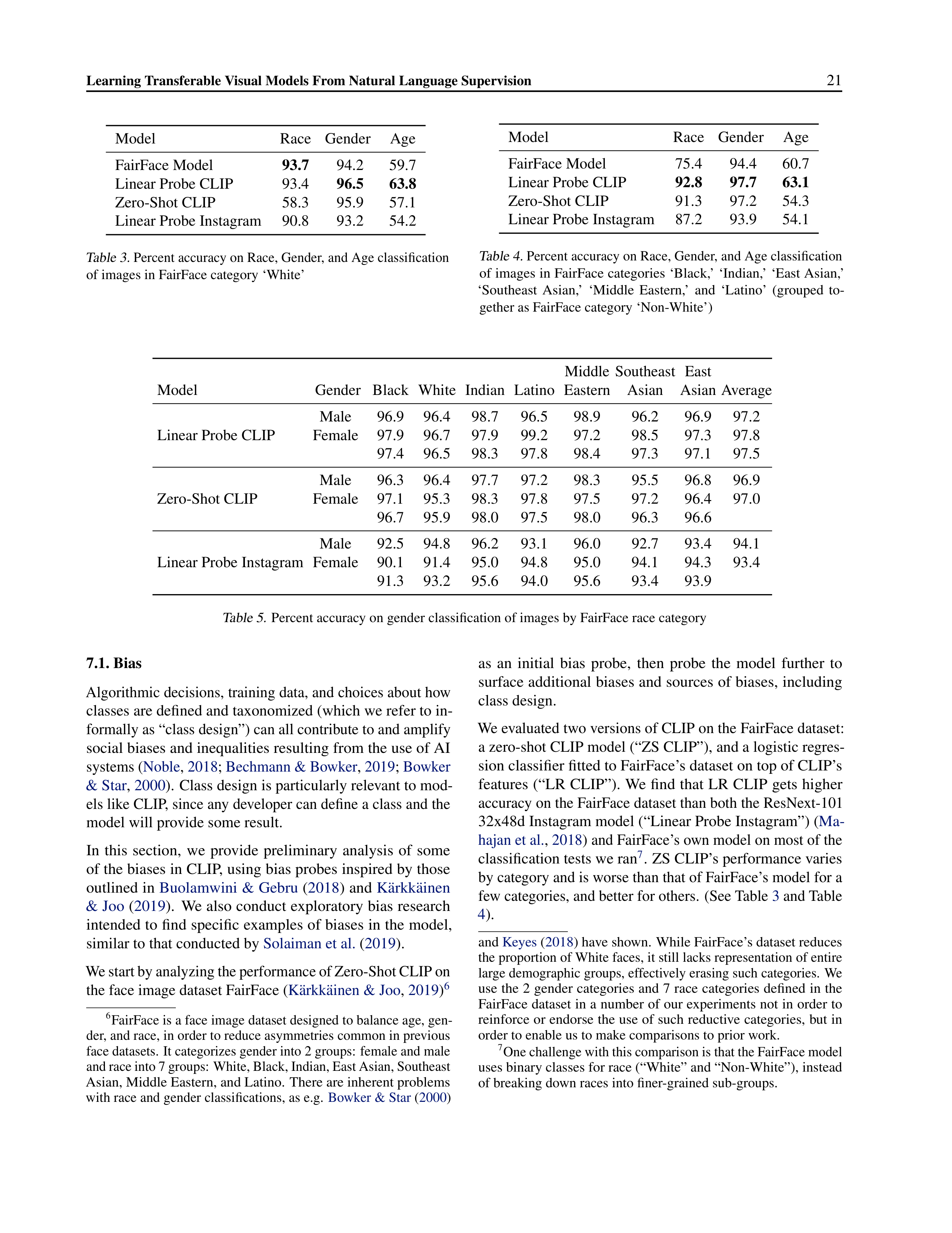
Learning Transferable Visual Models From Natural Language Supervision
21
Model
Race
Gender
Age
FairFace Model
93.7
94.2
59.7
Linear Probe CLIP
93.4
96.5
63.8
Zero-Shot CLIP
58.3
95.9
57.1
Linear Probe Instagram
90.8
93.2
54.2
Table 3.
Percent accuracy on Race, Gender, and Age classification
of images in FairFace category ‘White’
Model
Race
Gender
Age
FairFace Model
75.4
94.4
60.7
Linear Probe CLIP
92.8
97.7
63.1
Zero-Shot CLIP
91.3
97.2
54.3
Linear Probe Instagram
87.2
93.9
54.1
Table 4.
Percent accuracy on Race, Gender, and Age classification
of images in FairFace categories ‘Black,’ ‘Indian,’ ‘East Asian,’
‘Southeast
Asian,’
‘Middle
Eastern,’
and
‘Latino’
(grouped
to-
gether as FairFace category ‘Non-White’)
Middle
Southeast
East
Model
Gender
Black
White
Indian
Latino
Eastern
Asian
Asian
Average
Male
96.9
96.4
98.7
96.5
98.9
96.2
96.9
97.2
Linear Probe CLIP
Female
97.9
96.7
97.9
99.2
97.2
98.5
97.3
97.8
97.4
96.5
98.3
97.8
98.4
97.3
97.1
97.5
Male
96.3
96.4
97.7
97.2
98.3
95.5
96.8
96.9
Zero-Shot CLIP
Female
97.1
95.3
98.3
97.8
97.5
97.2
96.4
97.0
96.7
95.9
98.0
97.5
98.0
96.3
96.6
Male
92.5
94.8
96.2
93.1
96.0
92.7
93.4
94.1
Linear Probe Instagram
Female
90.1
91.4
95.0
94.8
95.0
94.1
94.3
93.4
91.3
93.2
95.6
94.0
95.6
93.4
93.9
Table 5.
Percent accuracy on gender classification of images by FairFace race category
7.1. Bias
Algorithmic decisions, training data, and choices about how
classes are defined and taxonomized (which we refer to in-
formally as “class design”) can all contribute to and amplify
social biases and inequalities resulting from the use of AI
systems (
Noble
,
2018
;
Bechmann & Bowker
,
2019
;
Bowker
& Star
,
2000
).
Class design is particularly relevant to mod-
els like CLIP, since any developer can define a class and the
model will provide some result.
In
this
section,
we
provide
preliminary
analysis
of
some
of the biases in CLIP, using bias probes inspired by those
outlined in
Buolamwini & Gebru
(
2018
) and
K
¨
arkk
¨
ainen
& Joo
(
2019
).
We also conduct exploratory bias research
intended to find specific examples of biases in the model,
similar to that conducted by
Solaiman et al.
(
2019
).
We start by analyzing the performance of Zero-Shot CLIP on
the face image dataset FairFace (
K
¨
arkk
¨
ainen & Joo
,
2019
)
6
6
FairFace is a face image dataset designed to balance age, gen-
der, and race, in order to reduce asymmetries common in previous
face datasets.
It categorizes gender into 2 groups:
female and male
and race into 7 groups: White, Black, Indian, East Asian, Southeast
Asian, Middle Eastern, and Latino.
There are inherent problems
with race and gender classifications, as e.g.
Bowker & Star
(
2000
)
as
an
initial
bias
probe,
then
probe
the
model
further
to
surface additional biases and sources of biases, including
class design.
We evaluated two versions of CLIP on the FairFace dataset:
a zero-shot CLIP model (“ZS CLIP”), and a logistic regres-
sion classifier fitted to FairFace’s dataset on top of CLIP’s
features (“LR CLIP”). We find that LR CLIP gets higher
accuracy on the FairFace dataset than both the ResNext-101
32x48d Instagram model (“Linear Probe Instagram”) (
Ma-
hajan et al.
,
2018
) and FairFace’s own model on most of the
classification tests we ran
7
.
ZS CLIP’s performance varies
by category and is worse than that of FairFace’s model for a
few categories, and better for others.
(See Table
3
and Table
4
).
and
Keyes
(
2018
) have shown.
While FairFace’s dataset reduces
the proportion of White faces, it still lacks representation of entire
large demographic groups, effectively erasing such categories.
We
use the 2 gender categories and 7 race categories defined in the
FairFace dataset in a number of our experiments not in order to
reinforce or endorse the use of such reductive categories, but in
order to enable us to make comparisons to prior work.
7
One challenge with this comparison is that the FairFace model
uses binary classes for race (“White” and “Non-White”), instead
of breaking down races into finer-grained sub-groups.
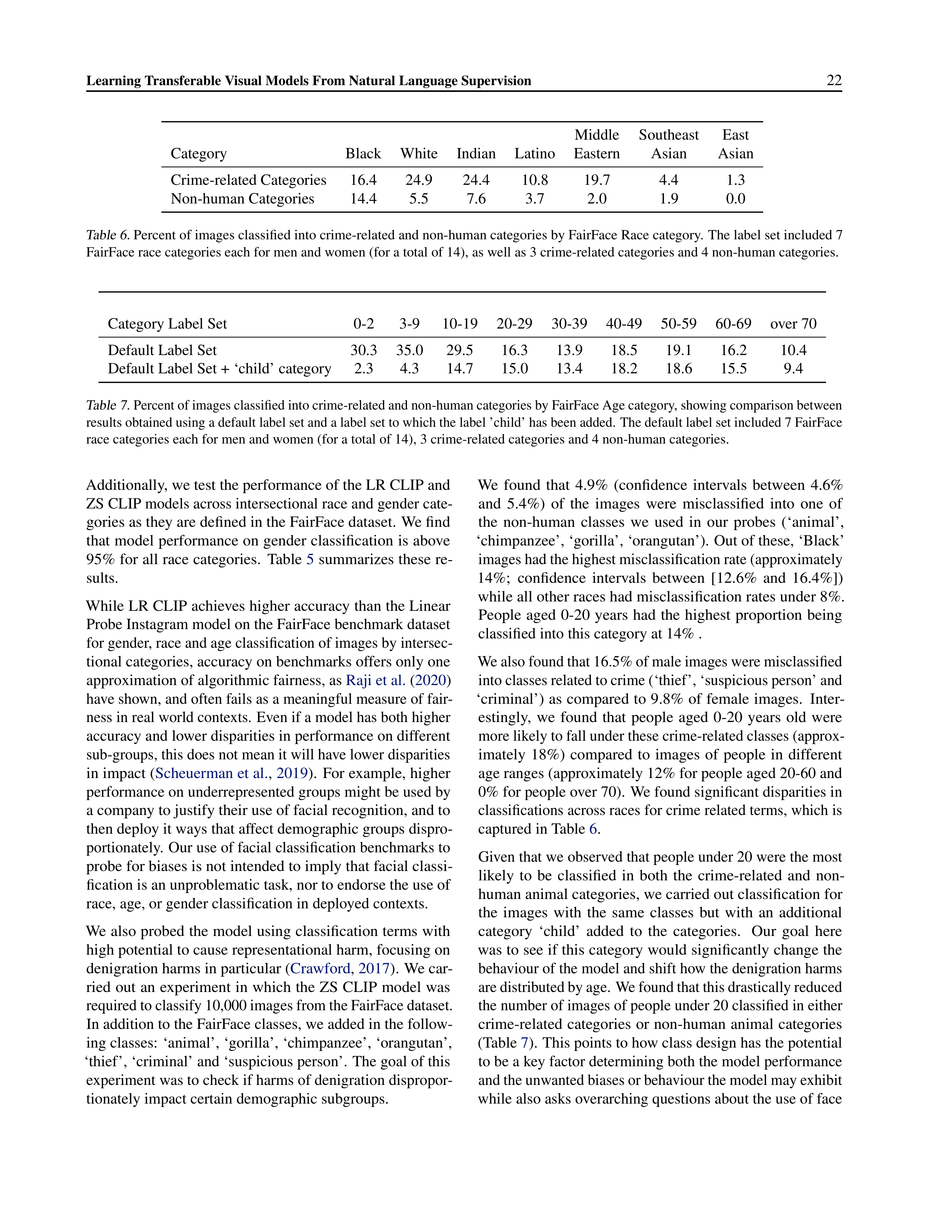
Learning Transferable Visual Models From Natural Language Supervision
22
Middle
Southeast
East
Category
Black
White
Indian
Latino
Eastern
Asian
Asian
Crime-related Categories
16.4
24.9
24.4
10.8
19.7
4.4
1.3
Non-human Categories
14.4
5.5
7.6
3.7
2.0
1.9
0.0
Table 6.
Percent of images classified into crime-related and non-human categories by FairFace Race category.
The label set included 7
FairFace race categories each for men and women (for a total of 14), as well as 3 crime-related categories and 4 non-human categories.
Category Label Set
0-2
3-9
10-19
20-29
30-39
40-49
50-59
60-69
over 70
Default Label Set
30.3
35.0
29.5
16.3
13.9
18.5
19.1
16.2
10.4
Default Label Set + ‘child’ category
2.3
4.3
14.7
15.0
13.4
18.2
18.6
15.5
9.4
Table 7.
Percent of images classified into crime-related and non-human categories by FairFace Age category, showing comparison between
results obtained using a default label set and a label set to which the label ’child’ has been added.
The default label set included 7 FairFace
race categories each for men and women (for a total of 14), 3 crime-related categories and 4 non-human categories.
Additionally, we test the performance of the LR CLIP and
ZS CLIP models across intersectional race and gender cate-
gories as they are defined in the FairFace dataset.
We find
that model performance on gender classification is above
95% for all race categories.
Table
5
summarizes these re-
sults.
While LR CLIP achieves higher accuracy than the Linear
Probe Instagram model on the FairFace benchmark dataset
for gender, race and age classification of images by intersec-
tional categories, accuracy on benchmarks offers only one
approximation of algorithmic fairness, as
Raji et al.
(
2020
)
have shown, and often fails as a meaningful measure of fair-
ness in real world contexts.
Even if a model has both higher
accuracy and lower disparities in performance on different
sub-groups, this does not mean it will have lower disparities
in impact (
Scheuerman et al.
,
2019
).
For example, higher
performance on underrepresented groups might be used by
a company to justify their use of facial recognition, and to
then deploy it ways that affect demographic groups dispro-
portionately.
Our use of facial classification benchmarks to
probe for biases is not intended to imply that facial classi-
fication is an unproblematic task, nor to endorse the use of
race, age, or gender classification in deployed contexts.
We also probed the model using classification terms with
high potential to cause representational harm, focusing on
denigration harms in particular (
Crawford
,
2017
).
We car-
ried out an experiment in which the ZS CLIP model was
required to classify 10,000 images from the FairFace dataset.
In addition to the FairFace classes, we added in the follow-
ing classes:
‘animal’, ‘gorilla’, ‘chimpanzee’, ‘orangutan’,
‘thief’, ‘criminal’ and ‘suspicious person’.
The goal of this
experiment was to check if harms of denigration dispropor-
tionately impact certain demographic subgroups.
We
found
that
4.9%
(confidence
intervals
between
4.6%
and
5.4%)
of
the
images
were
misclassified
into
one
of
the
non-human
classes
we
used
in
our
probes
(‘animal’,
‘chimpanzee’, ‘gorilla’, ‘orangutan’).
Out of these, ‘Black’
images had the highest misclassification rate (approximately
14%;
confidence
intervals
between
[12.6%
and
16.4%])
while all other races had misclassification rates under 8%.
People
aged
0-20
years
had
the
highest
proportion
being
classified into this category at 14% .
We also found that 16.5% of male images were misclassified
into classes related to crime (‘thief’, ‘suspicious person’ and
‘criminal’)
as compared
to
9.8% of
female
images.
Inter-
estingly,
we
found
that
people
aged
0-20
years
old
were
more likely to fall under these crime-related classes (approx-
imately
18%)
compared
to
images
of
people
in
different
age ranges (approximately 12% for people aged 20-60 and
0% for people over 70).
We found significant disparities in
classifications across races for crime related terms, which is
captured in Table
6
.
Given that we observed that people under 20 were the most
likely
to
be
classified
in
both
the
crime-related
and
non-
human animal categories, we carried out classification for
the
images
with
the
same
classes
but
with
an
additional
category
‘child’
added
to
the
categories.
Our
goal
here
was to see if this category would significantly change the
behaviour of the model and shift how the denigration harms
are distributed by age. We found that this drastically reduced
the number of images of people under 20 classified in either
crime-related
categories
or
non-human
animal
categories
(Table
7
).
This points to how class design has the potential
to be a key factor determining both the model performance
and the unwanted biases or behaviour the model may exhibit
while also asks overarching questions about the use of face
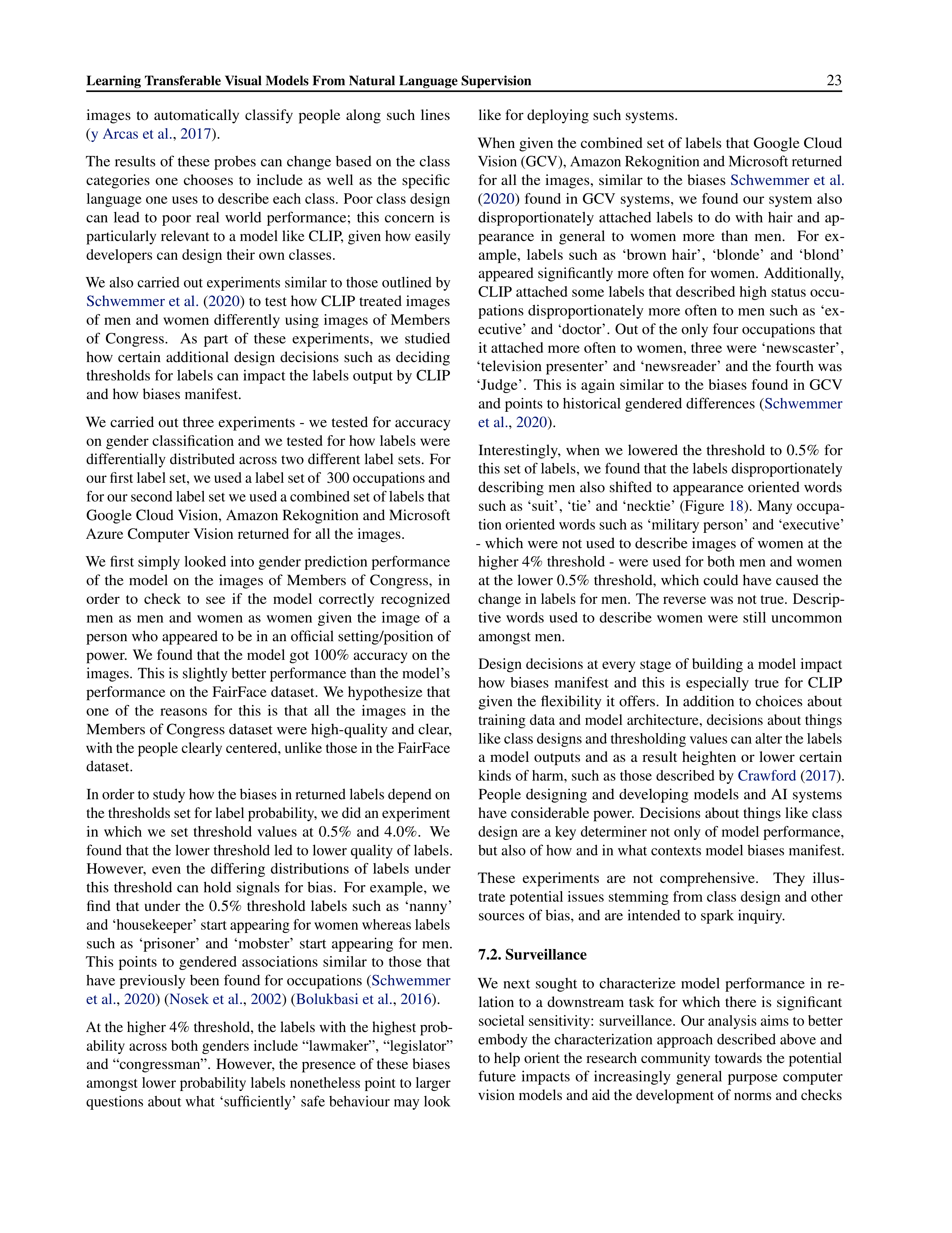
Learning Transferable Visual Models From Natural Language Supervision
23
images
to
automatically
classify
people
along
such
lines
(
y Arcas et al.
,
2017
).
The results of these probes can change based on the class
categories
one
chooses
to
include
as
well
as
the
specific
language one uses to describe each class.
Poor class design
can
lead
to
poor
real
world
performance;
this
concern
is
particularly relevant to a model like CLIP, given how easily
developers can design their own classes.
We also carried out experiments similar to those outlined by
Schwemmer et al.
(
2020
) to test how CLIP treated images
of men and women differently using images of Members
of
Congress.
As
part
of
these
experiments,
we
studied
how
certain
additional
design
decisions
such
as
deciding
thresholds for labels can impact the labels output by CLIP
and how biases manifest.
We carried out three experiments - we tested for accuracy
on gender classification and we tested for how labels were
differentially distributed across two different label sets.
For
our first label set, we used a label set of
300 occupations and
for our second label set we used a combined set of labels that
Google Cloud Vision, Amazon Rekognition and Microsoft
Azure Computer Vision returned for all the images.
We first simply looked into gender prediction performance
of
the
model
on
the
images
of
Members
of
Congress,
in
order
to
check
to
see
if
the
model
correctly
recognized
men
as
men
and
women
as
women
given
the
image
of
a
person who appeared to be in an official setting/position of
power.
We found that the model got 100% accuracy on the
images.
This is slightly better performance than the model’s
performance on the FairFace dataset.
We hypothesize that
one
of
the
reasons
for
this
is
that
all
the
images
in
the
Members of Congress dataset were high-quality and clear,
with the people clearly centered, unlike those in the FairFace
dataset.
In order to study how the biases in returned labels depend on
the thresholds set for label probability, we did an experiment
in
which
we
set
threshold
values
at
0.5%
and
4.0%.
We
found that the lower threshold led to lower quality of labels.
However,
even
the
differing
distributions
of
labels
under
this threshold can hold signals for bias.
For example, we
find
that
under
the
0.5%
threshold
labels
such
as
‘nanny’
and ‘housekeeper’ start appearing for women whereas labels
such
as
‘prisoner’
and
‘mobster’
start
appearing
for
men.
This
points
to
gendered
associations
similar
to
those
that
have previously been found for occupations (
Schwemmer
et al.
,
2020
) (
Nosek et al.
,
2002
) (
Bolukbasi et al.
,
2016
).
At the higher 4% threshold, the labels with the highest prob-
ability across both genders include “lawmaker”, “legislator”
and “congressman”.
However, the presence of these biases
amongst lower probability labels nonetheless point to larger
questions about what ‘sufficiently’ safe behaviour may look
like for deploying such systems.
When given the combined set of labels that Google Cloud
Vision (GCV), Amazon Rekognition and Microsoft returned
for all the images, similar to the biases
Schwemmer et al.
(
2020
) found in GCV systems, we found our system also
disproportionately attached labels to do with hair and ap-
pearance
in
general
to
women
more
than
men.
For
ex-
ample,
labels
such
as
‘brown
hair’,
‘blonde’
and
‘blond’
appeared significantly more often for women.
Additionally,
CLIP attached some labels that described high status occu-
pations disproportionately more often to men such as ‘ex-
ecutive’ and ‘doctor’.
Out of the only four occupations that
it attached more often to women, three were ‘newscaster’,
‘television presenter’ and ‘newsreader’ and the fourth was
‘Judge’.
This is again similar to the biases found in GCV
and points to historical gendered differences (
Schwemmer
et al.
,
2020
).
Interestingly, when we lowered the threshold to 0.5% for
this set of labels, we found that the labels disproportionately
describing men also shifted to appearance oriented words
such as ‘suit’, ‘tie’ and ‘necktie’ (Figure
18
).
Many occupa-
tion oriented words such as ‘military person’ and ‘executive’
- which were not used to describe images of women at the
higher 4% threshold - were used for both men and women
at the lower 0.5% threshold, which could have caused the
change in labels for men.
The reverse was not true.
Descrip-
tive words used to describe women were still uncommon
amongst men.
Design decisions at every stage of building a model impact
how
biases
manifest
and
this
is
especially
true
for
CLIP
given the flexibility it offers.
In addition to choices about
training data and model architecture, decisions about things
like class designs and thresholding values can alter the labels
a model outputs and as a result heighten or lower certain
kinds of harm, such as those described by
Crawford
(
2017
).
People designing and developing models and AI systems
have considerable power.
Decisions about things like class
design are a key determiner not only of model performance,
but also of how and in what contexts model biases manifest.
These
experiments
are
not
comprehensive.
They
illus-
trate potential issues stemming from class design and other
sources of bias, and are intended to spark inquiry.
7.2. Surveillance
We
next
sought
to
characterize
model
performance
in
re-
lation to a downstream task for which there is significant
societal sensitivity:
surveillance.
Our analysis aims to better
embody the characterization approach described above and
to help orient the research community towards the potential
future
impacts
of
increasingly
general
purpose
computer
vision models and aid the development of norms and checks
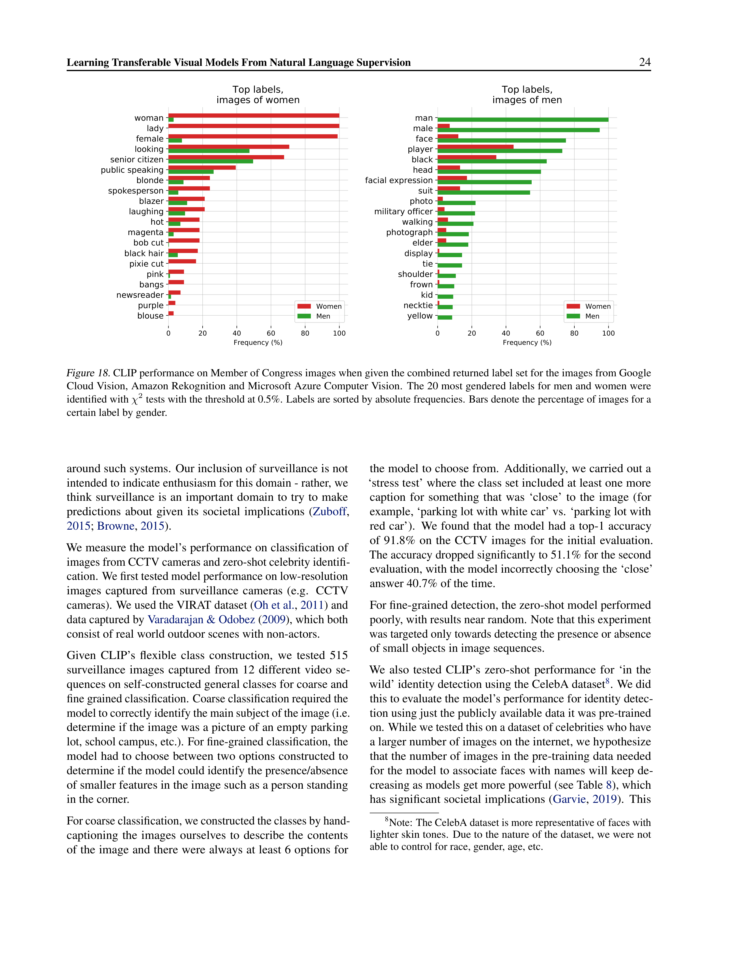
Learning Transferable Visual Models From Natural Language Supervision
24
0
20
40
60
80
100
Frequency (%)
blouse
purple
newsreader
bangs
pink
pixie cut
black hair
bob cut
magenta
hot
laughing
blazer
spokesperson
blonde
public speaking
senior citizen
looking
female
lady
woman
Top labels,
images of women
Women
Men
0
20
40
60
80
100
Frequency (%)
yellow
necktie
kid
frown
shoulder
tie
display
elder
photograph
walking
military officer
photo
suit
facial expression
head
black
player
face
male
man
Top labels,
images of men
Women
Men
Figure 18.
CLIP performance on Member of Congress images when given the combined returned label set for the images from Google
Cloud Vision, Amazon Rekognition and Microsoft Azure Computer Vision.
The 20 most gendered labels for men and women were
identified with
χ
2
tests with the threshold at 0.5%.
Labels are sorted by absolute frequencies.
Bars denote the percentage of images for a
certain label by gender.
around such systems.
Our inclusion of surveillance is not
intended to indicate enthusiasm for this domain - rather, we
think
surveillance
is
an
important
domain
to
try
to
make
predictions
about
given
its
societal
implications
(
Zuboff
,
2015
;
Browne
,
2015
).
We measure the model’s performance on classification of
images from CCTV cameras and zero-shot celebrity identifi-
cation.
We first tested model performance on low-resolution
images
captured
from
surveillance
cameras
(e.g.
CCTV
cameras).
We used the VIRAT dataset (
Oh et al.
,
2011
) and
data captured by
Varadarajan & Odobez
(
2009
), which both
consist of real world outdoor scenes with non-actors.
Given
CLIP’s
flexible
class
construction,
we
tested
515
surveillance
images
captured
from
12
different
video
se-
quences on self-constructed general classes for coarse and
fine grained classification.
Coarse classification required the
model to correctly identify the main subject of the image (i.e.
determine if the image was a picture of an empty parking
lot, school campus, etc.).
For fine-grained classification, the
model had to choose between two options constructed to
determine if the model could identify the presence/absence
of smaller features in the image such as a person standing
in the corner.
For coarse classification, we constructed the classes by hand-
captioning
the
images
ourselves
to
describe
the
contents
of the image and there were always at least 6 options for
the model to choose from.
Additionally, we carried out a
‘stress test’ where the class set included at least one more
caption
for
something
that
was
‘close’
to
the
image
(for
example, ‘parking lot with white car’ vs.
‘parking lot with
red
car’).
We
found
that
the
model
had
a
top-1
accuracy
of
91.8%
on
the
CCTV
images
for
the
initial
evaluation.
The accuracy dropped significantly to 51.1% for the second
evaluation, with the model incorrectly choosing the ‘close’
answer 40.7% of the time.
For fine-grained detection, the zero-shot model performed
poorly, with results near random.
Note that this experiment
was targeted only towards detecting the presence or absence
of small objects in image sequences.
We
also
tested
CLIP’s
zero-shot
performance
for
‘in
the
wild’ identity detection using the CelebA dataset
8
.
We did
this to evaluate the model’s performance for identity detec-
tion using just the publicly available data it was pre-trained
on.
While we tested this on a dataset of celebrities who have
a larger number of images on the internet, we hypothesize
that the number of images in the pre-training data needed
for the model to associate faces with names will keep de-
creasing as models get more powerful (see Table
8
), which
has significant societal implications (
Garvie
,
2019
).
This
8
Note:
The CelebA dataset is more representative of faces with
lighter skin tones.
Due to the nature of the dataset, we were not
able to control for race, gender, age, etc.
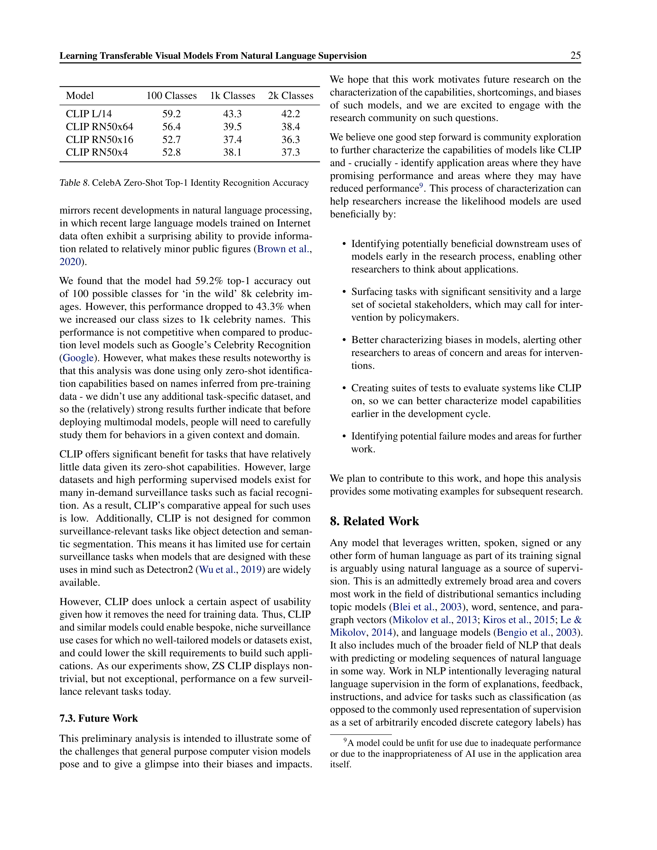
Learning Transferable Visual Models From Natural Language Supervision
25
Model
100 Classes
1k Classes
2k Classes
CLIP L/14
59.2
43.3
42.2
CLIP RN50x64
56.4
39.5
38.4
CLIP RN50x16
52.7
37.4
36.3
CLIP RN50x4
52.8
38.1
37.3
Table 8.
CelebA Zero-Shot Top-1 Identity Recognition Accuracy
mirrors recent developments in natural language processing,
in which recent large language models trained on Internet
data
often
exhibit
a
surprising
ability
to
provide
informa-
tion related to relatively minor public figures (
Brown et al.
,
2020
).
We
found
that
the
model
had
59.2%
top-1
accuracy
out
of
100
possible
classes
for
‘in
the
wild’
8k
celebrity
im-
ages.
However, this performance dropped to 43.3% when
we
increased
our
class
sizes
to
1k
celebrity
names.
This
performance is not competitive when compared to produc-
tion level models such as Google’s Celebrity Recognition
(
Google
).
However, what makes these results noteworthy is
that this analysis was done using only zero-shot identifica-
tion capabilities based on names inferred from pre-training
data - we didn’t use any additional task-specific dataset, and
so the (relatively) strong results further indicate that before
deploying multimodal models, people will need to carefully
study them for behaviors in a given context and domain.
CLIP offers significant benefit for tasks that have relatively
little data given its zero-shot capabilities.
However, large
datasets and high performing supervised models exist for
many in-demand surveillance tasks such as facial recogni-
tion.
As a result, CLIP’s comparative appeal for such uses
is
low.
Additionally,
CLIP
is
not
designed
for
common
surveillance-relevant tasks like object detection and seman-
tic segmentation.
This means it has limited use for certain
surveillance tasks when models that are designed with these
uses in mind such as Detectron2 (
Wu et al.
,
2019
) are widely
available.
However,
CLIP
does
unlock
a
certain
aspect
of
usability
given how it removes the need for training data.
Thus, CLIP
and similar models could enable bespoke, niche surveillance
use cases for which no well-tailored models or datasets exist,
and could lower the skill requirements to build such appli-
cations.
As our experiments show, ZS CLIP displays non-
trivial, but not exceptional, performance on a few surveil-
lance relevant tasks today.
7.3. Future Work
This preliminary analysis is intended to illustrate some of
the challenges that general purpose computer vision models
pose
and
to
give
a
glimpse
into
their
biases
and
impacts.
We
hope
that
this
work
motivates
future
research
on
the
characterization of the capabilities, shortcomings, and biases
of
such
models,
and
we
are
excited
to
engage
with
the
research community on such questions.
We believe one good step forward is community exploration
to further characterize the capabilities of models like CLIP
and - crucially - identify application areas where they have
promising
performance
and
areas
where
they
may
have
reduced performance
9
.
This process of characterization can
help
researchers
increase
the
likelihood
models
are
used
beneficially by:
•
Identifying potentially beneficial downstream uses of
models
early
in
the
research
process,
enabling
other
researchers to think about applications.
•
Surfacing tasks with significant sensitivity and a large
set of societal stakeholders, which may call for inter-
vention by policymakers.
•
Better characterizing biases in models, alerting other
researchers to areas of concern and areas for interven-
tions.
•
Creating suites of tests to evaluate systems like CLIP
on,
so
we
can
better
characterize
model
capabilities
earlier in the development cycle.
•
Identifying potential failure modes and areas for further
work.
We plan to contribute to this work, and hope this analysis
provides some motivating examples for subsequent research.
8. Related Work
Any
model
that
leverages
written,
spoken,
signed
or
any
other form of human language as part of its training signal
is arguably using natural language as a source of supervi-
sion.
This is an admittedly extremely broad area and covers
most work in the field of distributional semantics including
topic models (
Blei et al.
,
2003
), word, sentence, and para-
graph vectors (
Mikolov et al.
,
2013
;
Kiros et al.
,
2015
;
Le &
Mikolov
,
2014
), and language models (
Bengio et al.
,
2003
).
It also includes much of the broader field of NLP that deals
with predicting or modeling sequences of natural language
in some way.
Work in NLP intentionally leveraging natural
language supervision in the form of explanations, feedback,
instructions, and advice for tasks such as classification (as
opposed to the commonly used representation of supervision
as a set of arbitrarily encoded discrete category labels) has
9
A model could be unfit for use due to inadequate performance
or due to the inappropriateness of AI use in the application area
itself.
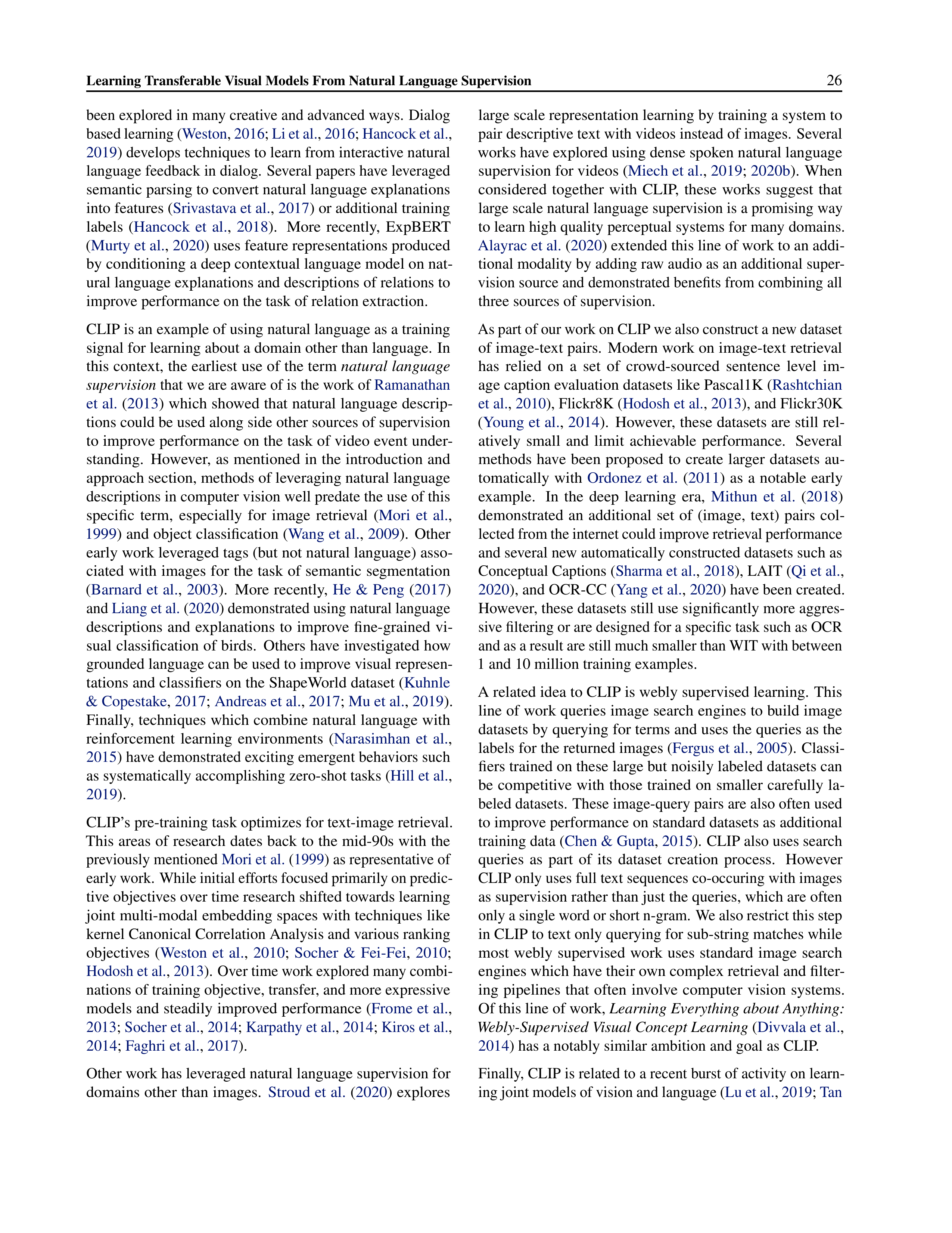
Learning Transferable Visual Models From Natural Language Supervision
26
been explored in many creative and advanced ways.
Dialog
based learning (
Weston
,
2016
;
Li et al.
,
2016
;
Hancock et al.
,
2019
) develops techniques to learn from interactive natural
language feedback in dialog.
Several papers have leveraged
semantic parsing to convert natural language explanations
into features (
Srivastava et al.
,
2017
) or additional training
labels
(
Hancock
et
al.
,
2018
).
More
recently,
ExpBERT
(
Murty et al.
,
2020
) uses feature representations produced
by conditioning a deep contextual language model on nat-
ural language explanations and descriptions of relations to
improve performance on the task of relation extraction.
CLIP is an example of using natural language as a training
signal for learning about a domain other than language.
In
this context, the earliest use of the term
natural language
supervision
that we are aware of is the work of
Ramanathan
et al.
(
2013
) which showed that natural language descrip-
tions could be used along side other sources of supervision
to improve performance on the task of video event under-
standing.
However,
as mentioned in the introduction and
approach section, methods of leveraging natural language
descriptions in computer vision well predate the use of this
specific
term,
especially
for
image
retrieval
(
Mori
et
al.
,
1999
) and object classification (
Wang et al.
,
2009
).
Other
early work leveraged tags (but not natural language) asso-
ciated with images for the task of semantic segmentation
(
Barnard
et
al.
,
2003
).
More
recently,
He
&
Peng
(
2017
)
and
Liang et al.
(
2020
) demonstrated using natural language
descriptions
and
explanations
to
improve
fine-grained
vi-
sual classification of birds.
Others have investigated how
grounded language can be used to improve visual represen-
tations and classifiers on the ShapeWorld dataset (
Kuhnle
& Copestake
,
2017
;
Andreas et al.
,
2017
;
Mu et al.
,
2019
).
Finally, techniques which combine natural language with
reinforcement
learning
environments
(
Narasimhan
et
al.
,
2015
) have demonstrated exciting emergent behaviors such
as systematically accomplishing zero-shot tasks (
Hill et al.
,
2019
).
CLIP’s pre-training task optimizes for text-image retrieval.
This areas of research dates back to the mid-90s with the
previously mentioned
Mori et al.
(
1999
) as representative of
early work. While initial efforts focused primarily on predic-
tive objectives over time research shifted towards learning
joint multi-modal embedding spaces with techniques like
kernel Canonical Correlation Analysis and various ranking
objectives
(
Weston
et
al.
,
2010
;
Socher
&
Fei-Fei
,
2010
;
Hodosh et al.
,
2013
).
Over time work explored many combi-
nations of training objective, transfer, and more expressive
models and steadily improved performance (
Frome et al.
,
2013
;
Socher et al.
,
2014
;
Karpathy et al.
,
2014
;
Kiros et al.
,
2014
;
Faghri et al.
,
2017
).
Other work has leveraged natural language supervision for
domains other than images.
Stroud et al.
(
2020
) explores
large scale representation learning by training a system to
pair descriptive text with videos instead of images.
Several
works have explored using dense spoken natural language
supervision for videos (
Miech et al.
,
2019
;
2020b
).
When
considered
together
with
CLIP,
these
works
suggest
that
large scale natural language supervision is a promising way
to learn high quality perceptual systems for many domains.
Alayrac et al.
(
2020
) extended this line of work to an addi-
tional modality by adding raw audio as an additional super-
vision source and demonstrated benefits from combining all
three sources of supervision.
As part of our work on CLIP we also construct a new dataset
of image-text pairs.
Modern work on image-text retrieval
has
relied
on
a
set
of
crowd-sourced
sentence
level
im-
age caption evaluation datasets like Pascal1K (
Rashtchian
et al.
,
2010
), Flickr8K (
Hodosh et al.
,
2013
), and Flickr30K
(
Young et al.
,
2014
).
However, these datasets are still rel-
atively
small
and
limit
achievable
performance.
Several
methods
have
been
proposed
to
create
larger
datasets
au-
tomatically
with
Ordonez
et
al.
(
2011
)
as
a
notable
early
example.
In
the
deep
learning
era,
Mithun
et
al.
(
2018
)
demonstrated
an
additional
set
of
(image,
text)
pairs
col-
lected from the internet could improve retrieval performance
and several new automatically constructed datasets such as
Conceptual Captions (
Sharma et al.
,
2018
), LAIT (
Qi et al.
,
2020
), and OCR-CC (
Yang et al.
,
2020
) have been created.
However, these datasets still use significantly more aggres-
sive filtering or are designed for a specific task such as OCR
and as a result are still much smaller than WIT with between
1 and 10 million training examples.
A related idea to CLIP is webly supervised learning.
This
line of work queries image search engines to build image
datasets by querying for terms and uses the queries as the
labels for the returned images (
Fergus et al.
,
2005
).
Classi-
fiers trained on these large but noisily labeled datasets can
be competitive with those trained on smaller carefully la-
beled datasets.
These image-query pairs are also often used
to improve performance on standard datasets as additional
training data (
Chen & Gupta
,
2015
).
CLIP also uses search
queries
as
part
of
its
dataset
creation
process.
However
CLIP only uses full text sequences co-occuring with images
as supervision rather than just the queries, which are often
only a single word or short n-gram.
We also restrict this step
in CLIP to text only querying for sub-string matches while
most
webly
supervised
work
uses
standard
image
search
engines which have their own complex retrieval and filter-
ing
pipelines
that
often
involve
computer
vision
systems.
Of this line of work,
Learning Everything about Anything:
Webly-Supervised Visual Concept Learning
(
Divvala et al.
,
2014
) has a notably similar ambition and goal as CLIP.
Finally, CLIP is related to a recent burst of activity on learn-
ing joint models of vision and language (
Lu et al.
,
2019
;
Tan
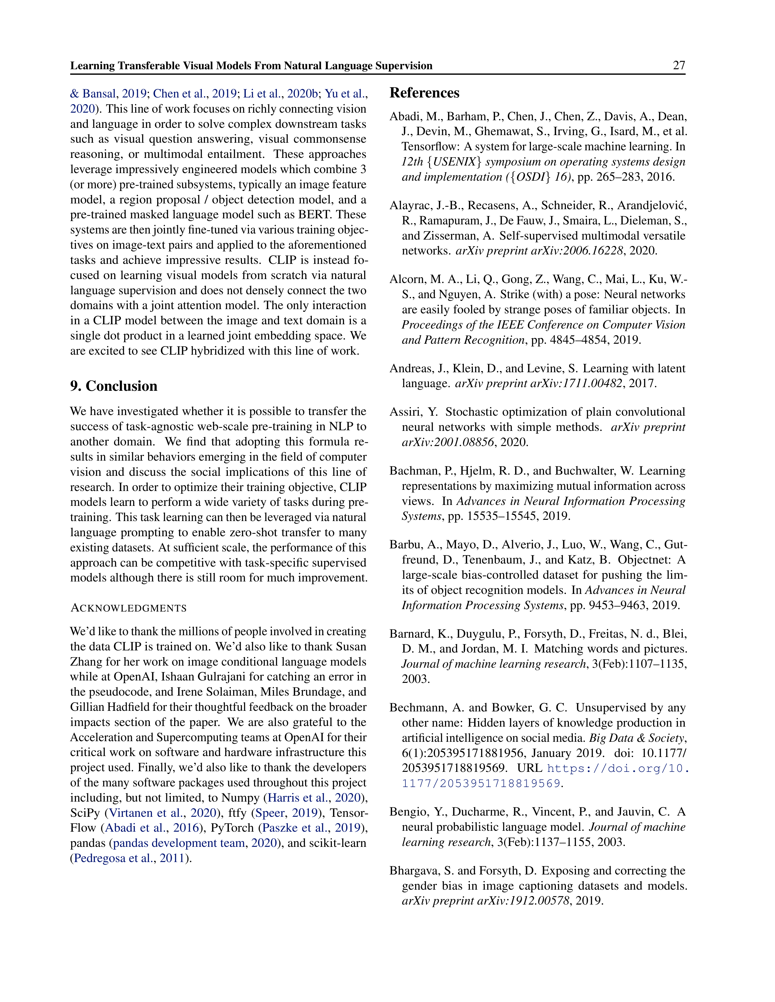
Learning Transferable Visual Models From Natural Language Supervision
27
& Bansal
,
2019
;
Chen et al.
,
2019
;
Li et al.
,
2020b
;
Yu et al.
,
2020
).
This line of work focuses on richly connecting vision
and language in order to solve complex downstream tasks
such
as
visual
question
answering,
visual
commonsense
reasoning,
or
multimodal
entailment.
These
approaches
leverage impressively engineered models which combine 3
(or more) pre-trained subsystems, typically an image feature
model,
a
region
proposal
/
object
detection
model,
and
a
pre-trained masked language model such as BERT. These
systems are then jointly fine-tuned via various training objec-
tives on image-text pairs and applied to the aforementioned
tasks
and
achieve
impressive
results.
CLIP
is
instead
fo-
cused
on
learning
visual
models
from
scratch
via
natural
language supervision and does not densely connect the two
domains with a joint attention model.
The only interaction
in a CLIP model between the image and text domain is a
single dot product in a learned joint embedding space.
We
are excited to see CLIP hybridized with this line of work.
9. Conclusion
We have investigated whether it is possible to transfer the
success of task-agnostic web-scale pre-training in NLP to
another
domain.
We
find
that
adopting
this
formula
re-
sults in similar behaviors emerging in the field of computer
vision
and
discuss
the
social
implications
of
this
line
of
research.
In order to optimize their training objective, CLIP
models learn to perform a wide variety of tasks during pre-
training.
This task learning can then be leveraged via natural
language
prompting
to
enable
zero-shot
transfer
to
many
existing datasets.
At sufficient scale, the performance of this
approach can be competitive with task-specific supervised
models although there is still room for much improvement.
A
CKNOWLEDGMENTS
We’d like to thank the millions of people involved in creating
the data CLIP is trained on.
We’d also like to thank Susan
Zhang for her work on image conditional language models
while at OpenAI, Ishaan Gulrajani for catching an error in
the pseudocode, and Irene Solaiman, Miles Brundage, and
Gillian Hadfield for their thoughtful feedback on the broader
impacts
section
of
the
paper.
We
are
also
grateful
to
the
Acceleration and Supercomputing teams at OpenAI for their
critical work on software and hardware infrastructure this
project used.
Finally, we’d also like to thank the developers
of the many software packages used throughout this project
including, but not limited, to Numpy (
Harris et al.
,
2020
),
SciPy
(
Virtanen
et
al.
,
2020
),
ftfy
(
Speer
,
2019
),
Tensor-
Flow
(
Abadi
et
al.
,
2016
),
PyTorch
(
Paszke
et
al.
,
2019
),
pandas (
pandas development team
,
2020
), and scikit-learn
(
Pedregosa et al.
,
2011
).
References
Abadi, M., Barham, P., Chen, J., Chen, Z., Davis, A., Dean,
J., Devin, M., Ghemawat, S., Irving, G., Isard, M., et al.
Tensorflow: A system for large-scale machine learning. In
12th
{
USENIX
}
symposium on operating systems design
and implementation (
{
OSDI
}
16)
, pp. 265–283, 2016.
Alayrac, J.-B., Recasens, A., Schneider, R., Arandjelovi
´
c,
R., Ramapuram, J., De Fauw, J., Smaira, L., Dieleman, S.,
and Zisserman, A.
Self-supervised multimodal versatile
networks.
arXiv preprint arXiv:2006.16228
, 2020.
Alcorn, M. A., Li, Q., Gong, Z., Wang, C., Mai, L., Ku, W.-
S., and Nguyen, A.
Strike (with) a pose:
Neural networks
are easily fooled by strange poses of familiar objects.
In
Proceedings of the IEEE Conference on Computer Vision
and Pattern Recognition
, pp. 4845–4854, 2019.
Andreas, J., Klein, D., and Levine, S.
Learning with latent
language.
arXiv preprint arXiv:1711.00482
, 2017.
Assiri,
Y.
Stochastic
optimization
of
plain
convolutional
neural
networks
with
simple
methods.
arXiv
preprint
arXiv:2001.08856
, 2020.
Bachman, P., Hjelm, R. D., and Buchwalter, W.
Learning
representations by maximizing mutual information across
views.
In
Advances
in
Neural
Information
Processing
Systems
, pp. 15535–15545, 2019.
Barbu, A., Mayo, D., Alverio, J., Luo, W., Wang, C., Gut-
freund,
D.,
Tenenbaum,
J.,
and
Katz,
B.
Objectnet:
A
large-scale
bias-controlled
dataset
for
pushing
the
lim-
its of object recognition models.
In
Advances in Neural
Information Processing Systems
, pp. 9453–9463, 2019.
Barnard, K., Duygulu, P., Forsyth, D., Freitas, N. d., Blei,
D. M., and Jordan, M. I.
Matching words and pictures.
Journal of machine learning research
, 3(Feb):1107–1135,
2003.
Bechmann,
A.
and
Bowker,
G.
C.
Unsupervised
by
any
other name:
Hidden layers of knowledge production in
artificial intelligence on social media.
Big Data & Society
,
6(1):205395171881956,
January
2019.
doi:
10.1177/
2053951718819569.
URL
https://doi.org/10.
1177/2053951718819569
.
Bengio,
Y.,
Ducharme,
R.,
Vincent,
P.,
and
Jauvin,
C.
A
neural probabilistic language model.
Journal of machine
learning research
, 3(Feb):1137–1155, 2003.
Bhargava, S. and Forsyth, D.
Exposing and correcting the
gender
bias
in
image
captioning
datasets
and
models.
arXiv preprint arXiv:1912.00578
, 2019.
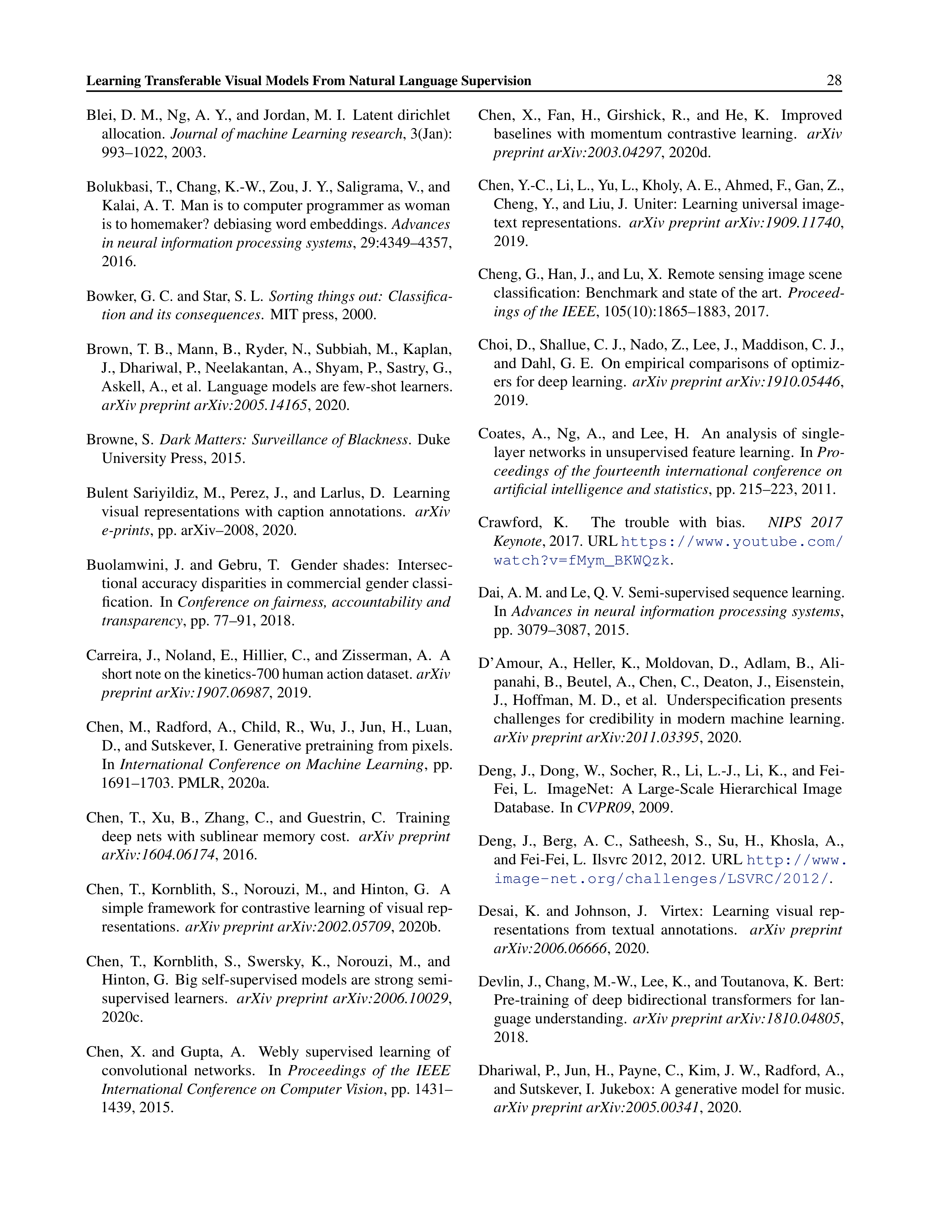
Learning Transferable Visual Models From Natural Language Supervision
28
Blei, D. M., Ng, A. Y., and Jordan, M. I.
Latent dirichlet
allocation.
Journal of machine Learning research
, 3(Jan):
993–1022, 2003.
Bolukbasi, T., Chang, K.-W., Zou, J. Y., Saligrama, V., and
Kalai, A. T.
Man is to computer programmer as woman
is to homemaker?
debiasing word embeddings.
Advances
in neural information processing systems
, 29:4349–4357,
2016.
Bowker, G. C. and Star, S. L.
Sorting things out:
Classifica-
tion and its consequences
.
MIT press, 2000.
Brown, T. B., Mann, B., Ryder, N., Subbiah, M., Kaplan,
J., Dhariwal, P., Neelakantan, A., Shyam, P., Sastry, G.,
Askell, A., et al.
Language models are few-shot learners.
arXiv preprint arXiv:2005.14165
, 2020.
Browne, S.
Dark Matters:
Surveillance of Blackness
.
Duke
University Press, 2015.
Bulent Sariyildiz,
M.,
Perez,
J.,
and Larlus,
D.
Learning
visual
representations
with
caption
annotations.
arXiv
e-prints
, pp. arXiv–2008, 2020.
Buolamwini,
J.
and
Gebru,
T.
Gender
shades:
Intersec-
tional accuracy disparities in commercial gender classi-
fication.
In
Conference on fairness, accountability and
transparency
, pp. 77–91, 2018.
Carreira, J., Noland, E., Hillier, C., and Zisserman, A.
A
short note on the kinetics-700 human action dataset.
arXiv
preprint arXiv:1907.06987
, 2019.
Chen,
M.,
Radford,
A.,
Child,
R.,
Wu,
J.,
Jun,
H.,
Luan,
D., and Sutskever, I.
Generative pretraining from pixels.
In
International
Conference
on
Machine
Learning
,
pp.
1691–1703. PMLR, 2020a.
Chen,
T.,
Xu,
B.,
Zhang,
C.,
and
Guestrin,
C.
Training
deep
nets
with
sublinear
memory
cost.
arXiv
preprint
arXiv:1604.06174
, 2016.
Chen,
T.,
Kornblith,
S.,
Norouzi,
M.,
and
Hinton,
G.
A
simple framework for contrastive learning of visual rep-
resentations.
arXiv preprint arXiv:2002.05709
, 2020b.
Chen,
T.,
Kornblith,
S.,
Swersky,
K.,
Norouzi,
M.,
and
Hinton, G.
Big self-supervised models are strong semi-
supervised
learners.
arXiv
preprint
arXiv:2006.10029
,
2020c.
Chen,
X.
and
Gupta,
A.
Webly
supervised
learning
of
convolutional
networks.
In
Proceedings
of
the
IEEE
International Conference on Computer Vision
, pp. 1431–
1439, 2015.
Chen,
X.,
Fan,
H.,
Girshick,
R.,
and
He,
K.
Improved
baselines
with
momentum
contrastive
learning.
arXiv
preprint arXiv:2003.04297
, 2020d.
Chen, Y.-C., Li, L., Yu, L., Kholy, A. E., Ahmed, F., Gan, Z.,
Cheng, Y., and Liu, J.
Uniter:
Learning universal image-
text representations.
arXiv preprint arXiv:1909.11740
,
2019.
Cheng, G., Han, J., and Lu, X.
Remote sensing image scene
classification:
Benchmark and state of the art.
Proceed-
ings of the IEEE
, 105(10):1865–1883, 2017.
Choi, D., Shallue, C. J., Nado, Z., Lee, J., Maddison, C. J.,
and Dahl, G. E.
On empirical comparisons of optimiz-
ers for deep learning.
arXiv preprint arXiv:1910.05446
,
2019.
Coates,
A.,
Ng,
A.,
and
Lee,
H.
An
analysis
of
single-
layer networks in unsupervised feature learning.
In
Pro-
ceedings
of
the
fourteenth
international
conference
on
artificial intelligence and statistics
, pp. 215–223, 2011.
Crawford,
K.
The
trouble
with
bias.
NIPS
2017
Keynote
, 2017. URL
https://www.youtube.com/
watch?v=fMym_BKWQzk
.
Dai, A. M. and Le, Q. V. Semi-supervised sequence learning.
In
Advances
in
neural
information
processing
systems
,
pp. 3079–3087, 2015.
D’Amour,
A.,
Heller,
K.,
Moldovan,
D.,
Adlam,
B.,
Ali-
panahi, B., Beutel, A., Chen, C., Deaton, J., Eisenstein,
J.,
Hoffman,
M.
D.,
et
al.
Underspecification
presents
challenges
for
credibility
in
modern
machine
learning.
arXiv preprint arXiv:2011.03395
, 2020.
Deng,
J.,
Dong,
W., Socher,
R.,
Li,
L.-J.,
Li,
K.,
and Fei-
Fei,
L.
ImageNet:
A
Large-Scale
Hierarchical
Image
Database.
In
CVPR09
, 2009.
Deng,
J.,
Berg,
A.
C.,
Satheesh,
S.,
Su,
H.,
Khosla,
A.,
and Fei-Fei, L.
Ilsvrc 2012, 2012.
URL
http://www.
image-net.org/challenges/LSVRC/2012/
.
Desai,
K.
and
Johnson,
J.
Virtex:
Learning
visual
rep-
resentations
from
textual
annotations.
arXiv
preprint
arXiv:2006.06666
, 2020.
Devlin, J., Chang, M.-W., Lee, K., and Toutanova, K.
Bert:
Pre-training
of
deep
bidirectional
transformers
for
lan-
guage understanding.
arXiv preprint arXiv:1810.04805
,
2018.
Dhariwal, P., Jun, H., Payne, C., Kim, J. W., Radford, A.,
and Sutskever, I.
Jukebox:
A generative model for music.
arXiv preprint arXiv:2005.00341
, 2020.
Learning Transferable Visual Models From Natural Language Supervision
29
Divvala,
S.
K.,
Farhadi,
A.,
and
Guestrin,
C.
Learning
everything about anything:
Webly-supervised visual con-
cept
learning.
In
Proceedings
of
the
IEEE
Conference
on Computer Vision and Pattern Recognition
, pp. 3270–
3277, 2014.
Dodge, S. and Karam, L.
A study and comparison of human
and deep learning recognition performance under visual
distortions.
In
2017
26th
international
conference
on
computer communication and networks (ICCCN)
, pp. 1–
7. IEEE, 2017.
Dosovitskiy,
A.,
Beyer,
L.,
Kolesnikov,
A.,
Weissenborn,
D., Zhai, X., Unterthiner, T., Dehghani, M., Minderer, M.,
Heigold, G., Gelly, S., et al.
An image is worth 16x16
words: Transformers for image recognition at scale.
arXiv
preprint arXiv:2010.11929
, 2020.
Elhoseiny, M., Saleh, B., and Elgammal, A.
Write a classi-
fier:
Zero-shot learning using purely textual descriptions.
In
Proceedings of the IEEE International Conference on
Computer Vision
, pp. 2584–2591, 2013.
Faghri, F., Fleet, D. J., Kiros, J. R., and Fidler, S. Vse++: Im-
proving visual-semantic embeddings with hard negatives.
arXiv preprint arXiv:1707.05612
, 2017.
Fergus, R., Fei-Fei, L., Perona, P., and Zisserman, A.
Learn-
ing
object
categories
from
google’s
image
search.
In
Tenth IEEE International Conference on Computer Vision
(ICCV’05)
Volume
1
,
volume
2,
pp.
1816–1823.
IEEE,
2005.
Frome, A., Corrado, G. S., Shlens, J., Bengio, S., Dean, J.,
Ranzato,
M.,
and
Mikolov,
T.
Devise:
A
deep
visual-
semantic embedding model.
In
Advances in neural infor-
mation processing systems
, pp. 2121–2129, 2013.
Gan, Z., Chen, Y.-C., Li, L., Zhu, C., Cheng, Y., and Liu, J.
Large-scale adversarial training for vision-and-language
representation learning.
arXiv preprint arXiv:2006.06195
,
2020.
Gao, T., Fisch, A., and Chen, D.
Making pre-trained lan-
guage
models
better
few-shot
learners.
arXiv
preprint
arXiv:2012.15723
, 2020.
Garvie,
C.,
May
2019.
URL
https://www.
flawedfacedata.com/
.
Geiger,
A.,
Lenz,
P.,
and
Urtasun,
R.
Are
we
ready
for
autonomous driving?
the kitti vision benchmark suite.
In
Conference on Computer Vision and Pattern Recognition
(CVPR)
, 2012.
Geirhos, R., Rubisch, P., Michaelis, C., Bethge, M., Wich-
mann, F. A., and Brendel, W.
Imagenet-trained cnns are
biased towards texture; increasing shape bias improves ac-
curacy and robustness.
arXiv preprint arXiv:1811.12231
,
2018.
Geirhos,
R.,
Jacobsen,
J.-H.,
Michaelis,
C.,
Zemel,
R.,
Brendel,
W.,
Bethge,
M.,
and
Wichmann,
F.
A.
Short-
cut
learning
in
deep
neural
networks.
arXiv
preprint
arXiv:2004.07780
, 2020.
Gomez, L., Patel, Y., Rusi
˜
nol, M., Karatzas, D., and Jawahar,
C.
Self-supervised
learning
of
visual
features
through
embedding images into text topic spaces.
In
Proceedings
of the IEEE Conference on Computer Vision and Pattern
Recognition
, pp. 4230–4239, 2017.
Goodfellow,
I.
J.,
Shlens,
J.,
and
Szegedy,
C.
Explain-
ing and harnessing adversarial examples.
arXiv preprint
arXiv:1412.6572
, 2014.
Goodfellow,
I.
J.,
Erhan,
D.,
Carrier,
P.
L.,
Courville,
A.,
Mirza, M., Hamner, B., Cukierski, W., Tang, Y., Thaler,
D., Lee, D.-H., et al.
Challenges in representation learn-
ing:
A report on three machine learning contests.
Neural
Networks
, 64:59–63, 2015.
Google.
Google
cloud
api:
Celebrity
recognition.
URL
https://cloud.google.com/vision/docs/
celebrity-recognition
.
Griewank, A. and Walther, A.
Algorithm 799:
revolve:
an
implementation
of
checkpointing
for
the
reverse
or
ad-
joint mode of computational differentiation.
ACM Trans-
actions on Mathematical Software (TOMS)
, 26(1):19–45,
2000.
Grill,
J.-B.,
Strub,
F.,
Altch
´
e,
F.,
Tallec,
C.,
Richemond,
P. H.,
Buchatskaya,
E.,
Doersch,
C.,
Pires,
B. A.,
Guo,
Z. D., Azar, M. G., et al.
Bootstrap your own latent:
A
new approach to self-supervised learning.
arXiv preprint
arXiv:2006.07733
, 2020.
Ha,
D.,
Dai,
A.,
and
Le,
Q.
V.
Hypernetworks.
arXiv
preprint arXiv:1609.09106
, 2016.
Hancock, B., Bringmann, M., Varma, P., Liang, P., Wang,
S., and R
´
e, C.
Training classifiers with natural language
explanations.
In
Proceedings of the conference. Associ-
ation
for
Computational
Linguistics.
Meeting
,
volume
2018, pp. 1884. NIH Public Access, 2018.
Hancock,
B.,
Bordes,
A.,
Mazare,
P.-E.,
and
Weston,
J.
Learning from dialogue after deployment:
Feed yourself,
chatbot!
arXiv preprint arXiv:1901.05415
, 2019.
Harris, C. R., Millman, K. J., van der Walt, S. J., Gommers,
R., Virtanen, P., Cournapeau, D., Wieser, E., Taylor, J.,
Berg, S., Smith, N. J., Kern, R., Picus, M., Hoyer, S., van
Kerkwijk, M. H., Brett, M., Haldane, A., Fern
´
andez del
Learning Transferable Visual Models From Natural Language Supervision
30
R
´
ıo,
J.,
Wiebe,
M.,
Peterson,
P.,
G
´
erard-Marchant,
P.,
Sheppard,
K.,
Reddy,
T.,
Weckesser,
W.,
Abbasi,
H.,
Gohlke,
C.,
and
Oliphant,
T.
E.
Array
programming
with NumPy.
Nature
, 585:357–362, 2020.
doi:
10.1038/
s41586-020-2649-2.
Hays, J. and Efros, A. A.
Im2gps:
estimating geographic
information
from
a
single
image.
In
2008
ieee
confer-
ence on computer vision and pattern recognition
, pp. 1–8.
IEEE, 2008.
He,
K.,
Zhang,
X.,
Ren,
S.,
and
Sun,
J.
Delving
deep
into rectifiers:
Surpassing human-level performance on
imagenet classification.
In
Proceedings of the IEEE inter-
national conference on computer vision
, pp. 1026–1034,
2015.
He, K., Zhang, X., Ren, S., and Sun, J.
Deep residual learn-
ing for image recognition.
In
Proceedings of the IEEE
conference on computer vision and pattern recognition
,
pp. 770–778, 2016a.
He, K., Zhang, X., Ren, S., and Sun, J.
Deep residual learn-
ing for image recognition.
In
Proceedings of the IEEE
conference on computer vision and pattern recognition
,
pp. 770–778, 2016b.
He,
K.,
Fan,
H.,
Wu,
Y.,
Xie,
S.,
and
Girshick,
R.
Mo-
mentum contrast for unsupervised visual representation
learning.
In
Proceedings of the IEEE/CVF Conference
on Computer Vision and Pattern Recognition
, pp. 9729–
9738, 2020.
He, T., Zhang, Z., Zhang, H., Zhang, Z., Xie, J., and Li, M.
Bag of tricks for image classification with convolutional
neural networks.
In
Proceedings of the IEEE Conference
on Computer Vision and Pattern Recognition
, pp. 558–
567, 2019.
He, X. and Peng, Y.
Fine-grained image classification via
combining vision and language.
In
Proceedings of the
IEEE Conference on Computer Vision and Pattern Recog-
nition
, pp. 5994–6002, 2017.
Helber, P., Bischke, B., Dengel, A., and Borth, D.
Eurosat:
A
novel
dataset
and
deep
learning
benchmark
for
land
use
and
land
cover
classification.
IEEE
Journal
of
Se-
lected Topics in Applied Earth Observations and Remote
Sensing
, 12(7):2217–2226, 2019.
Henaff, O. Data-efficient image recognition with contrastive
predictive coding.
In
International Conference on Ma-
chine Learning
, pp. 4182–4192. PMLR, 2020.
Hendrycks,
D.
and
Dietterich,
T.
Benchmarking
neural
network robustness to common corruptions and perturba-
tions.
arXiv preprint arXiv:1903.12261
, 2019.
Hendrycks, D. and Gimpel, K.
Gaussian error linear units
(gelus).
arXiv preprint arXiv:1606.08415
, 2016.
Hendrycks,
D.,
Zhao,
K.,
Basart,
S.,
Steinhardt,
J.,
and
Song, D.
Natural adversarial examples.
arXiv preprint
arXiv:1907.07174
, 2019.
Hendrycks, D., Basart, S., Mu, N., Kadavath, S., Wang, F.,
Dorundo,
E.,
Desai,
R.,
Zhu,
T.,
Parajuli,
S.,
Guo,
M.,
et
al.
The
many
faces
of
robustness:
A
critical
analy-
sis of out-of-distribution generalization.
arXiv preprint
arXiv:2006.16241
, 2020a.
Hendrycks, D., Liu, X., Wallace, E., Dziedzic, A., Krishnan,
R., and Song, D.
Pretrained transformers improve out-of-
distribution robustness.
arXiv preprint arXiv:2004.06100
,
2020b.
Hestness, J., Narang, S., Ardalani, N., Diamos, G., Jun, H.,
Kianinejad, H., Patwary, M., Ali, M., Yang, Y., and Zhou,
Y. Deep learning scaling is predictable, empirically.
arXiv
preprint arXiv:1712.00409
, 2017.
Hill, F., Lampinen, A., Schneider, R., Clark, S., Botvinick,
M.,
McClelland,
J. L.,
and Santoro,
A.
Environmental
drivers of systematicity and generalization in a situated
agent.
In
International Conference on Learning Repre-
sentations
, 2019.
Hodosh, M., Young, P., and Hockenmaier, J.
Framing image
description as a ranking task: Data, models and evaluation
metrics.
Journal of Artificial Intelligence Research
, 47:
853–899, 2013.
Hongsuck Seo, P., Weyand, T., Sim, J., and Han, B.
Cplanet:
Enhancing image geolocalization by combinatorial parti-
tioning of maps.
In
Proceedings of the European Confer-
ence on Computer Vision (ECCV)
, pp. 536–551, 2018.
Howard,
J.
and
Ruder,
S.
Universal
language
model
fine-tuning
for
text
classification.
arXiv
preprint
arXiv:1801.06146
, 2018.
Ilyas,
A.,
Santurkar,
S.,
Tsipras,
D.,
Engstrom,
L.,
Tran,
B.,
and
Madry,
A.
Adversarial
examples
are
not
bugs,
they
are
features.
In
Advances
in
Neural
Information
Processing Systems
, pp. 125–136, 2019.
Ioffe, S. and Szegedy, C.
Batch normalization:
Accelerating
deep network training by reducing internal covariate shift.
arXiv preprint arXiv:1502.03167
, 2015.
Jaderberg, M., Simonyan, K., Vedaldi, A., and Zisserman,
A.
Deep structured output learning for unconstrained text
recognition.
arXiv preprint arXiv:1412.5903
, 2014.
Jaderberg, M., Simonyan, K., Zisserman, A., et al.
Spatial
transformer networks.
Advances in neural information
processing systems
, 28:2017–2025, 2015.
Learning Transferable Visual Models From Natural Language Supervision
31
Johnson, J., Hariharan, B., van der Maaten, L., Fei-Fei, L.,
Lawrence Zitnick,
C.,
and Girshick,
R.
Clevr:
A diag-
nostic dataset for compositional language and elementary
visual
reasoning.
In
Proceedings
of
the
IEEE
Confer-
ence
on
Computer
Vision
and
Pattern
Recognition
,
pp.
2901–2910, 2017.
Joulin, A., Van Der Maaten, L., Jabri, A., and Vasilache, N.
Learning
visual
features
from
large
weakly
supervised
data.
In
European Conference on Computer Vision
, pp.
67–84. Springer, 2016.
Kalfaoglu, M., Kalkan, S., and Alatan, A. A.
Late temporal
modeling
in
3d
cnn
architectures
with
bert
for
action
recognition.
arXiv preprint arXiv:2008.01232
, 2020.
Kaplan,
J.,
McCandlish,
S.,
Henighan,
T.,
Brown,
T.
B.,
Chess, B., Child, R., Gray, S., Radford, A., Wu, J., and
Amodei,
D.
Scaling
laws
for
neural
language
models.
arXiv preprint arXiv:2001.08361
, 2020.
Karpathy, A., Joulin, A., and Fei-Fei, L. F.
Deep fragment
embeddings
for
bidirectional
image
sentence
mapping.
In
Advances
in
neural
information
processing
systems
,
pp. 1889–1897, 2014.
Keyes, O.
The misgendering machines:
Trans/hci implica-
tions of automatic gender recognition.
Proceedings of the
ACM on Human-Computer Interaction
, 2(CSCW):1–22,
2018.
Kiela, D., Firooz, H., Mohan, A., Goswami, V., Singh, A.,
Ringshia,
P.,
and
Testuggine,
D.
The
hateful
memes
challenge:
Detecting hate speech in multimodal memes.
arXiv preprint arXiv:2005.04790
, 2020.
Kingma, D. P. and Ba, J.
Adam:
A method for stochastic
optimization.
arXiv preprint arXiv:1412.6980
, 2014.
Kiros,
R.,
Salakhutdinov,
R.,
and
Zemel,
R.
S.
Unifying
visual-semantic embeddings with multimodal neural lan-
guage models.
arXiv preprint arXiv:1411.2539
, 2014.
Kiros, R., Zhu, Y., Salakhutdinov, R. R., Zemel, R., Urtasun,
R.,
Torralba,
A.,
and
Fidler,
S.
Skip-thought
vectors.
Advances in neural information processing systems
, 28:
3294–3302, 2015.
Kolesnikov,
A.,
Beyer,
L.,
Zhai,
X.,
Puigcerver,
J.,
Yung,
J.,
Gelly,
S.,
and
Houlsby,
N.
Large
scale
learning
of
general visual representations for transfer.
arXiv preprint
arXiv:1912.11370
, 2019.
Kornblith, S., Shlens, J., and Le, Q. V.
Do better imagenet
models
transfer
better?
In
Proceedings
of
the
IEEE
conference on computer vision and pattern recognition
,
pp. 2661–2671, 2019.
Krishna,
R.,
Zhu,
Y.,
Groth,
O.,
Johnson,
J.,
Hata,
K.,
Kravitz, J., Chen, S., Kalantidis, Y., Li, L.-J., Shamma,
D. A., et al.
Visual genome:
Connecting language and
vision using crowdsourced dense image annotations.
In-
ternational
journal
of
computer
vision
,
123(1):32–73,
2017.
Krizhevsky, A., Sutskever, I., and Hinton, G. E.
Imagenet
classification with deep convolutional neural networks.
In
Advances
in
neural
information
processing
systems
,
pp. 1097–1105, 2012.
Kuhnle,
A.
and
Copestake,
A.
Shapeworld-a
new
test
methodology
for
multimodal
language
understanding.
arXiv preprint arXiv:1704.04517
, 2017.
K
¨
arkk
¨
ainen, K. and Joo, J.
Fairface:
Face attribute dataset
for balanced race, gender, and age, 2019.
Lake, B. M., Ullman, T. D., Tenenbaum, J. B., and Gersh-
man,
S. J.
Building machines that learn and think like
people, 2016.
Lampert, C. H., Nickisch, H., and Harmeling, S.
Learning
to detect unseen object classes by between-class attribute
transfer.
In
2009 IEEE Conference on Computer Vision
and Pattern Recognition
, pp. 951–958. IEEE, 2009.
Larochelle, H., Erhan, D., and Bengio, Y. Zero-data learning
of new tasks.
2008.
Le, Q. and Mikolov, T.
Distributed representations of sen-
tences
and
documents.
In
International
conference
on
machine learning
, pp. 1188–1196, 2014.
LeCun,
Y.
The
mnist
database
of
handwritten
digits.
http://yann. lecun. com/exdb/mnist/
.
Lee,
D.-H.
Pseudo-label:
The
simple
and
efficient
semi-
supervised learning method for deep neural networks.
Lei Ba,
J.,
Swersky,
K.,
Fidler,
S.,
et al.
Predicting deep
zero-shot
convolutional
neural
networks
using
textual
descriptions.
In
Proceedings of the IEEE International
Conference on Computer Vision
, pp. 4247–4255, 2015.
Li, A., Jabri, A., Joulin, A., and van der Maaten, L. Learning
visual
n-grams
from
web
data.
In
Proceedings
of
the
IEEE International Conference on Computer Vision
, pp.
4183–4192, 2017.
Li,
G.,
Duan,
N.,
Fang,
Y.,
Gong,
M.,
and
Jiang,
D.
Unicoder-vl: A universal encoder for vision and language
by cross-modal pre-training.
2020a.
Li, J., Miller, A. H., Chopra, S., Ranzato, M., and Weston, J.
Learning through dialogue interactions by asking ques-
tions.
arXiv preprint arXiv:1612.04936
, 2016.
Learning Transferable Visual Models From Natural Language Supervision
32
Li, X., Yin, X., Li, C., Hu, X., Zhang, P., Zhang, L., Wang,
L.,
Hu,
H.,
Dong,
L.,
Wei,
F.,
et
al.
Oscar:
Object-
semantics aligned pre-training for vision-language tasks.
arXiv preprint arXiv:2004.06165
, 2020b.
Liang, W., Zou, J., and Yu, Z.
Alice:
Active learning with
contrastive natural language explanations.
arXiv preprint
arXiv:2009.10259
, 2020.
Lin, T.-Y., Maire, M., Belongie, S., Hays, J., Perona, P., Ra-
manan, D., Doll
´
ar, P., and Zitnick, C. L.
Microsoft coco:
Common objects in context.
In
European conference on
computer vision
, pp. 740–755. Springer, 2014.
Linzen,
T.
How
can
we
accelerate
progress
towards
human-like
linguistic
generalization?
arXiv
preprint
arXiv:2005.00955
, 2020.
Lippe,
P.,
Holla,
N.,
Chandra,
S.,
Rajamanickam,
S.,
An-
toniou, G., Shutova, E., and Yannakoudakis, H.
A mul-
timodal framework for the detection of hateful memes.
arXiv preprint arXiv:2012.12871
, 2020.
Liu,
P.
J.,
Saleh,
M.,
Pot,
E.,
Goodrich,
B.,
Sepa-
ssi,
R.,
Kaiser,
L.,
and
Shazeer,
N.
Generating
wikipedia by summarizing long sequences.
arXiv preprint
arXiv:1801.10198
, 2018.
Locatello,
F.,
Bauer,
S.,
Lucic,
M.,
R
¨
atsch,
G.,
Gelly,
S.,
Sch
¨
olkopf,
B.,
and
Bachem,
O.
A
sober
look
at
the
unsupervised
learning
of
disentangled
representations
and their evaluation.
arXiv preprint arXiv:2010.14766
,
2020.
Loshchilov,
I.
and
Hutter,
F.
Sgdr:
Stochastic
gra-
dient
descent
with
warm
restarts.
arXiv
preprint
arXiv:1608.03983
, 2016.
Loshchilov, I. and Hutter, F.
Decoupled weight decay regu-
larization.
arXiv preprint arXiv:1711.05101
, 2017.
Lu, J., Batra, D., Parikh, D., and Lee, S.
Vilbert:
Pretraining
task-agnostic
visiolinguistic
representations
for
vision-
and-language tasks.
In
Advances in Neural Information
Processing Systems
, pp. 13–23, 2019.
Lu, Z., Xiong, X., Li, Y., Stroud, J., and Ross, D. Leveraging
weakly supervised data and pose representation for action
recognition,
2020.
URL
https://www.youtube.
com/watch?v=KOQFxbPPLOE&t=1390s
.
Lucic, M., Kurach, K., Michalski, M., Gelly, S., and Bous-
quet,
O.
Are
gans
created
equal?
a
large-scale
study.
Advances in neural information processing systems
, 31:
700–709, 2018.
Mahajan, D., Girshick, R., Ramanathan, V., He, K., Paluri,
M.,
Li,
Y.,
Bharambe,
A.,
and
van
der
Maaten,
L.
Ex-
ploring the limits of weakly supervised pretraining.
In
Proceedings of the European Conference on Computer
Vision (ECCV)
, pp. 181–196, 2018.
McCann,
B.,
Bradbury,
J.,
Xiong,
C.,
and
Socher,
R.
Learned in translation:
Contextualized word vectors.
In
Advances in neural information processing systems
, pp.
6294–6305, 2017.
McCann, B., Keskar, N. S., Xiong, C., and Socher, R.
The
natural language decathlon:
Multitask learning as ques-
tion answering.
arXiv preprint arXiv:1806.08730
, 2018.
Micikevicius, P., Narang, S., Alben, J., Diamos, G., Elsen,
E., Garcia, D., Ginsburg, B., Houston, M., Kuchaiev, O.,
Venkatesh,
G.,
et
al.
Mixed
precision
training.
arXiv
preprint arXiv:1710.03740
, 2017.
Miech, A., Zhukov, D., Alayrac, J.-B., Tapaswi, M., Laptev,
I., and Sivic, J.
Howto100m:
Learning a text-video em-
bedding by watching hundred million narrated video clips.
In
Proceedings of the IEEE international conference on
computer vision
, pp. 2630–2640, 2019.
Miech, A., Alayrac, J.-B., Laptev, I., Sivic, J., and Zisser-
man, A.
Rareact:
A video dataset of unusual interactions.
arXiv preprint arXiv:2008.01018
, 2020a.
Miech, A., Alayrac, J.-B., Smaira, L., Laptev, I., Sivic, J.,
and Zisserman, A. End-to-end learning of visual represen-
tations from uncurated instructional videos.
In
Proceed-
ings of the IEEE/CVF Conference on Computer Vision
and Pattern Recognition
, pp. 9879–9889, 2020b.
Mikolov,
T.,
Sutskever,
I.,
Chen,
K.,
Corrado,
G.
S.,
and
Dean, J.
Distributed representations of words and phrases
and their compositionality.
Advances in neural informa-
tion processing systems
, 26:3111–3119, 2013.
Miller, J., Krauth, K., Recht, B., and Schmidt, L.
The effect
of natural distribution shift on question answering models.
arXiv preprint arXiv:2004.14444
, 2020.
Mishra, A., Alahari, K., and Jawahar, C.
Scene text recogni-
tion using higher order language priors.
2012.
Mithun,
N.
C.,
Panda,
R.,
Papalexakis,
E.
E.,
and
Roy-
Chowdhury, A. K.
Webly supervised joint embedding for
cross-modal image-text retrieval.
In
Proceedings of the
26th ACM international conference on Multimedia
, pp.
1856–1864, 2018.
Mori, Y., Takahashi, H., and Oka, R.
Image-to-word trans-
formation based on dividing and vector quantizing images
with words.
Citeseer, 1999.
Mu, J., Liang, P., and Goodman, N. Shaping visual represen-
tations with language for few-shot classification.
arXiv
preprint arXiv:1911.02683
, 2019.
Learning Transferable Visual Models From Natural Language Supervision
33
Muller-Budack, E., Pustu-Iren, K., and Ewerth, R.
Geolo-
cation
estimation
of
photos
using
a
hierarchical
model
and scene classification.
In
Proceedings of the European
Conference on Computer Vision (ECCV)
, pp. 563–579,
2018.
Murty, S., Koh, P. W., and Liang, P. Expbert: Representation
engineering with natural language explanations.
arXiv
preprint arXiv:2005.01932
, 2020.
Narasimhan, K., Kulkarni, T., and Barzilay, R.
Language
understanding for text-based games using deep reinforce-
ment learning.
arXiv preprint arXiv:1506.08941
, 2015.
Netzer,
Y.,
Wang,
T.,
Coates,
A.,
Bissacco,
A.,
Wu,
B.,
and
Ng,
A.
Y.
Reading
digits
in
natural
images
with
unsupervised feature learning.
2011.
Noble, S. U.
Algorithms of oppression: How search engines
reinforce racism.
2018.
Nosek, B. A., Banaji, M. R., and Greenwald, A. G.
Harvest-
ing implicit group attitudes and beliefs from a demonstra-
tion web site.
Group Dynamics:
Theory, Research, and
Practice
, 6(1):101, 2002.
Oh, S., Hoogs, A., Perera, A., Cuntoor, N., Chen, C.-C., Lee,
J. T., Mukherjee, S., Aggarwal, J., Lee, H., Davis, L., et al.
A large-scale benchmark dataset for event recognition in
surveillance video.
In
CVPR 2011
, pp. 3153–3160. IEEE,
2011.
Oliver, A., Odena, A., Raffel, C. A., Cubuk, E. D., and Good-
fellow, I.
Realistic evaluation of deep semi-supervised
learning algorithms.
Advances in neural information pro-
cessing systems
, 31:3235–3246, 2018.
Oord, A. v. d., Li, Y., and Vinyals, O.
Representation learn-
ing
with
contrastive
predictive
coding.
arXiv
preprint
arXiv:1807.03748
, 2018.
Ordonez, V., Kulkarni, G., and Berg, T.
Im2text: Describing
images using 1 million captioned photographs.
Advances
in neural information processing systems
, 24:1143–1151,
2011.
pandas
development
team,
T.
pandas-dev/pandas:
Pan-
das,
February
2020.
URL
https://doi.org/10.
5281/zenodo.3509134
.
Parkhi,
O.
M.,
Vedaldi,
A.,
Zisserman,
A.,
and
Jawahar,
C. V.
Cats and dogs.
In
IEEE Conference on Computer
Vision and Pattern Recognition
, 2012.
Paszke,
A.,
Gross,
S.,
Massa,
F.,
Lerer,
A.,
Bradbury,
J.,
Chanan, G., Killeen, T., Lin, Z., Gimelshein, N., Antiga,
L., Desmaison, A., Kopf, A., Yang, E., DeVito, Z., Raison,
M.,
Tejani,
A.,
Chilamkurthy,
S.,
Steiner,
B.,
Fang,
L.,
Bai,
J.,
and
Chintala,
S.
Pytorch:
An
imperative
style,
high-performance
deep
learning
library.
In
Advances
in Neural Information Processing Systems 32
, pp. 8024–
8035, 2019.
Pedregosa,
F.,
Varoquaux,
G.,
Gramfort,
A.,
Michel,
V.,
Thirion,
B.,
Grisel,
O.,
Blondel,
M.,
Prettenhofer,
P.,
Weiss, R., Dubourg, V., Vanderplas, J., Passos, A., Cour-
napeau, D., Brucher, M., Perrot, M., and Duchesnay, E.
Scikit-learn:
Machine
learning
in
Python.
Journal
of
Machine Learning Research
, 12:2825–2830, 2011.
Pennington,
J.,
Socher,
R.,
and
Manning,
C.
D.
Glove:
Global vectors for word representation.
In
Proceedings
of the 2014 conference on empirical methods in natural
language processing (EMNLP)
, pp. 1532–1543, 2014.
Peters, M. E., Neumann, M., Iyyer, M., Gardner, M., Clark,
C.,
Lee,
K.,
and
Zettlemoyer,
L.
Deep
contextualized
word representations.
arXiv preprint arXiv:1802.05365
,
2018.
Qi,
D.,
Su,
L.,
Song,
J.,
Cui,
E.,
Bharti,
T.,
and
Sacheti,
A.
Imagebert:
Cross-modal
pre-training
with
large-
scale weak-supervised image-text data.
arXiv preprint
arXiv:2001.07966
, 2020.
Quattoni, A., Collins, M., and Darrell, T.
Learning visual
representations using images with captions. In
2007 IEEE
Conference on Computer Vision and Pattern Recognition
,
pp. 1–8. IEEE, 2007.
Radford, A., Narasimhan, K., Salimans, T., and Sutskever,
I.
Improving language understanding by generative pre-
training, 2018.
Radford, A., Wu, J., Child, R., Luan, D., Amodei, D., and
Sutskever, I. Language models are unsupervised multitask
learners.
2019.
Raffel,
C.,
Shazeer,
N.,
Roberts,
A.,
Lee,
K.,
Narang,
S.,
Matena, M., Zhou, Y., Li, W., and Liu, P. J.
Exploring
the limits of transfer learning with a unified text-to-text
transformer.
arXiv preprint arXiv:1910.10683
, 2019.
Raji,
I.
D.,
Gebru,
T.,
Mitchell,
M.,
Buolamwini,
J.,
Lee,
J., and Denton, E.
Saving face:
Investigating the ethical
concerns of facial recognition auditing, 2020.
Ramanathan,
V.,
Liang,
P.,
and
Fei-Fei,
L.
Video
event
understanding
using
natural
language
descriptions.
In
Proceedings
of
the
IEEE
International
Conference
on
Computer Vision
, pp. 905–912, 2013.
Rashtchian, C., Young, P., Hodosh, M., and Hockenmaier, J.
Collecting image annotations using amazon’s mechanical
turk.
In
Proceedings of the NAACL HLT 2010 Workshop
on Creating Speech and Language Data with Amazon’s
Mechanical Turk
, pp. 139–147, 2010.
Learning Transferable Visual Models From Natural Language Supervision
34
Recht, B., Roelofs, R., Schmidt, L., and Shankar, V.
Do im-
agenet classifiers generalize to imagenet?
arXiv preprint
arXiv:1902.10811
, 2019.
Salimans, T. and Kingma, D. P.
Weight normalization:
A
simple reparameterization to accelerate training of deep
neural networks.
In
Advances in neural information pro-
cessing systems
, pp. 901–909, 2016.
Scheuerman, M. K., Paul, J. M., and Brubaker, J. R.
How
computers see gender:
An evaluation of gender classifica-
tion in commercial facial analysis services.
Proceedings
of the ACM on Human-Computer Interaction
, 3(CSCW):
1–33, 2019.
Schwemmer, C., Knight, C., Bello-Pardo, E. D., Oklobdzija,
S.,
Schoonvelde,
M.,
and
Lockhart,
J.
W.
Diagnosing
gender
bias
in
image
recognition
systems.
Socius
,
6:
2378023120967171, 2020.
Sennrich, R., Haddow, B., and Birch, A.
Neural machine
translation
of
rare
words
with
subword
units.
arXiv
preprint arXiv:1508.07909
, 2015.
Shankar, V., Dave, A., Roelofs, R., Ramanan, D., Recht, B.,
and Schmidt, L.
Do image classifiers generalize across
time?
arXiv preprint arXiv:1906.02168
, 2019.
Sharma, P., Ding, N., Goodman, S., and Soricut, R.
Con-
ceptual captions:
A cleaned, hypernymed, image alt-text
dataset for automatic image captioning.
In
Proceedings
of the 56th Annual Meeting of the Association for Compu-
tational Linguistics (Volume 1:
Long Papers)
, pp. 2556–
2565, 2018.
Singh,
A.,
Natarajan,
V.,
Shah,
M.,
Jiang,
Y.,
Chen,
X.,
Batra,
D.,
Parikh,
D.,
and
Rohrbach,
M.
Towards
vqa
models that can read.
In
Proceedings of the IEEE Con-
ference on Computer Vision and Pattern Recognition
, pp.
8317–8326, 2019.
Socher,
R. and Fei-Fei,
L.
Connecting modalities:
Semi-
supervised segmentation and annotation of images using
unaligned text corpora.
In
2010 IEEE Computer Society
Conference on Computer Vision and Pattern Recognition
,
pp. 966–973. IEEE, 2010.
Socher,
R.,
Perelygin,
A.,
Wu,
J.,
Chuang,
J.,
Manning,
C. D., Ng, A. Y., and Potts, C.
Recursive deep models for
semantic compositionality over a sentiment treebank.
In
Proceedings of the 2013 conference on empirical methods
in natural language processing
, pp. 1631–1642, 2013.
Socher, R., Karpathy, A., Le, Q. V., Manning, C. D., and Ng,
A. Y.
Grounded compositional semantics for finding and
describing
images
with
sentences.
Transactions
of
the
Association
for
Computational
Linguistics
,
2:207–218,
2014.
Sohn, K.
Improved deep metric learning with multi-class
n-pair loss objective.
In
Advances in neural information
processing systems
, pp. 1857–1865, 2016.
Solaiman, I., Brundage, M., Clark, J., Askell, A., Herbert-
Voss, A., Wu, J., Radford, A., Krueger, G., Kim, J. W.,
Kreps,
S.,
McCain,
M.,
Newhouse,
A.,
Blazakis,
J.,
McGuffie,
K.,
and Wang,
J.
Release strategies and the
social impacts of language models, 2019.
Soomro, K., Zamir, A. R., and Shah, M.
Ucf101:
A dataset
of
101
human
actions
classes
from
videos
in
the
wild.
arXiv preprint arXiv:1212.0402
, 2012.
Speer, R.
ftfy.
Zenodo, 2019.
URL
https://doi.org/
10.5281/zenodo.2591652
.
Version 5.5.
Srivastava, N. and Salakhutdinov, R.
Multimodal learning
with deep boltzmann machines.
In
NIPS
, 2012.
Srivastava, S., Labutov, I., and Mitchell, T.
Joint concept
learning and semantic parsing from natural language ex-
planations.
In
Proceedings
of
the
2017
conference
on
empirical
methods
in
natural
language
processing
,
pp.
1527–1536, 2017.
Stallkamp, J., Schlipsing, M., Salmen, J., and Igel, C.
The
German Traffic Sign Recognition Benchmark:
A multi-
class classification competition.
In
IEEE International
Joint
Conference
on
Neural
Networks
,
pp.
1453–1460,
2011.
Stroud, J. C., Ross, D. A., Sun, C., Deng, J., Sukthankar, R.,
and Schmid, C.
Learning video representations from tex-
tual web supervision.
arXiv preprint arXiv:2007.14937
,
2020.
Szegedy,
C.,
Ioffe,
S.,
Vanhoucke,
V.,
and
Alemi,
A.
Inception-v4,
inception-resnet
and
the
impact
of
residual
connections
on
learning.
arXiv
preprint
arXiv:1602.07261
, 2016.
Tan, H. and Bansal, M.
Lxmert:
Learning cross-modality
encoder representations from transformers.
arXiv preprint
arXiv:1908.07490
, 2019.
Tan,
M.
and
Le,
Q.
V.
Efficientnet:
Rethinking
model
scaling for convolutional neural networks.
arXiv preprint
arXiv:1905.11946
, 2019.
Taori,
R.,
Dave,
A.,
Shankar,
V.,
Carlini,
N.,
Recht,
B.,
and
Schmidt,
L.
Measuring
robustness
to
natural
dis-
tribution
shifts
in
image
classification.
arXiv
preprint
arXiv:2007.00644
, 2020.
Thomee, B., Shamma, D. A., Friedland, G., Elizalde, B., Ni,
K., Poland, D., Borth, D., and Li, L.-J.
Yfcc100m:
The
new data in multimedia research.
Communications of the
ACM
, 59(2):64–73, 2016.
Learning Transferable Visual Models From Natural Language Supervision
35
Tian, Y., Krishnan, D., and Isola, P.
Contrastive multiview
coding.
arXiv preprint arXiv:1906.05849
, 2019.
Tian,
Y.,
Wang,
Y.,
Krishnan,
D.,
Tenenbaum,
J.
B.,
and
Isola,
P.
Rethinking
few-shot
image
classification:
a
good
embedding
is
all
you
need?
arXiv
preprint
arXiv:2003.11539
, 2020.
Torralba, A., Fergus, R., and Freeman, W. T.
80 million tiny
images:
A
large
data
set
for
nonparametric
object
and
scene recognition.
IEEE transactions on pattern analysis
and machine intelligence
, 30(11):1958–1970, 2008.
Touvron,
H.,
Vedaldi,
A.,
Douze,
M.,
and J
´
egou,
H.
Fix-
ing the train-test resolution discrepancy.
In
Advances in
neural information processing systems
, pp. 8252–8262,
2019.
Varadarajan, J. and Odobez, J.-M.
Topic models for scene
analysis and abnormality detection.
In
2009 IEEE 12th
International Conference on Computer Vision Workshops,
ICCV Workshops
, pp. 1338–1345. IEEE, 2009.
Vaswani, A., Shazeer, N., Parmar, N., Uszkoreit, J., Jones,
L., Gomez, A. N., Kaiser,
Ł
., and Polosukhin, I.
Atten-
tion is all you need.
In
Advances in neural information
processing systems
, pp. 5998–6008, 2017.
Veeling,
B.
S.,
Linmans,
J.,
Winkens,
J.,
Cohen,
T.,
and
Welling, M.
Rotation equivariant CNNs for digital pathol-
ogy.
June 2018.
Virtanen, P., Gommers, R., Oliphant, T. E., Haberland, M.,
Reddy,
T.,
Cournapeau,
D.,
Burovski,
E.,
Peterson,
P.,
Weckesser, W., Bright, J., van der Walt, S. J., Brett, M.,
Wilson, J., Millman, K. J., Mayorov, N., Nelson, A. R. J.,
Jones,
E.,
Kern,
R.,
Larson,
E.,
Carey,
C.
J.,
Polat,
˙
I.,
Feng,
Y.,
Moore,
E.
W.,
VanderPlas,
J.,
Laxalde,
D.,
Perktold, J., Cimrman, R., Henriksen, I., Quintero, E. A.,
Harris, C. R., Archibald, A. M., Ribeiro, A. H., Pedregosa,
F., van Mulbregt, P., and SciPy 1.0 Contributors.
SciPy
1.0:
Fundamental Algorithms for Scientific Computing
in
Python.
Nature
Methods
,
17:261–272,
2020.
doi:
10.1038/s41592-019-0686-2.
Vo, N., Jacobs, N., and Hays, J.
Revisiting im2gps in the
deep learning era.
In
Proceedings of the IEEE Interna-
tional Conference on Computer Vision
, pp. 2621–2630,
2017.
Wang,
A.,
Singh,
A.,
Michael,
J.,
Hill,
F.,
Levy,
O.,
and
Bowman, S. R.
Glue:
A multi-task benchmark and anal-
ysis platform for natural language understanding.
arXiv
preprint arXiv:1804.07461
, 2018.
Wang, H., Ge, S., Lipton, Z., and Xing, E. P.
Learning ro-
bust global representations by penalizing local predictive
power.
In
Advances in Neural Information Processing
Systems
, pp. 10506–10518, 2019.
Wang, H., Lu, P., Zhang, H., Yang, M., Bai, X., Xu, Y., He,
M., Wang, Y., and Liu, W.
All you need is boundary:
To-
ward arbitrary-shaped text spotting.
In
Proceedings of the
AAAI Conference on Artificial Intelligence
,
volume 34,
pp. 12160–12167, 2020.
Wang, J., Markert, K., and Everingham, M.
Learning mod-
els for object recognition from natural language descrip-
tions.
In
BMVC
, volume 1, pp.
2, 2009.
Weston,
J.,
Bengio,
S.,
and
Usunier,
N.
Large
scale
im-
age annotation:
learning to rank with joint word-image
embeddings.
Machine learning
, 81(1):21–35, 2010.
Weston, J. E.
Dialog-based language learning.
In
Advances
in Neural Information Processing Systems
, pp. 829–837,
2016.
Weyand, T., Kostrikov, I., and Philbin, J. Planet-photo geolo-
cation with convolutional neural networks.
In
European
Conference
on
Computer
Vision
,
pp.
37–55.
Springer,
2016.
Wu,
Y.,
Kirillov,
A.,
Massa,
F.,
Lo,
W.-Y.,
and
Gir-
shick,
R.
Detectron2.
https://github.com/
facebookresearch/detectron2
, 2019.
Wu, Z., Xiong, Y., Yu, S., and Lin, D.
Unsupervised feature
learning via non-parametric instance-level discrimination.
arXiv preprint arXiv:1805.01978
, 2018.
Xie, Q., Luong, M.-T., Hovy, E., and Le, Q. V.
Self-training
with noisy student improves imagenet classification.
In
Proceedings of the IEEE/CVF Conference on Computer
Vision and Pattern Recognition
, pp. 10687–10698, 2020.
y
Arcas,
B.
A.,
Mitchell,
M.,
and
Todorov,
A.
Physiognomy’s
new
clothes.
2017.
URL
https://medium.com/@blaisea/
physiognomys-new-clothes-f2d4b59fdd6a
.
Yang,
Z.,
Lu,
Y.,
Wang,
J.,
Yin,
X.,
Florencio,
D.,
Wang,
L., Zhang, C., Zhang, L., and Luo, J.
Tap:
Text-aware
pre-training for text-vqa and text-caption.
arXiv preprint
arXiv:2012.04638
, 2020.
Yogatama,
D.,
d’Autume,
C.
d.
M.,
Connor,
J.,
Kocisky,
T., Chrzanowski, M., Kong, L., Lazaridou, A., Ling, W.,
Yu, L., Dyer, C., et al.
Learning and evaluating general
linguistic intelligence.
arXiv preprint arXiv:1901.11373
,
2019.
Young, P., Lai, A., Hodosh, M., and Hockenmaier, J.
From
image descriptions to visual denotations:
New similarity
metrics
for
semantic
inference
over
event
descriptions.
Transactions of the Association for Computational Lin-
guistics
, 2:67–78, 2014.
Learning Transferable Visual Models From Natural Language Supervision
36
Yu,
F.,
Tang,
J.,
Yin,
W.,
Sun,
Y.,
Tian,
H.,
Wu,
H.,
and
Wang,
H.
Ernie-vil:
Knowledge
enhanced
vision-
language
representations
through
scene
graph.
arXiv
preprint arXiv:2006.16934
, 2020.
Zeiler, M. D. and Fergus, R.
Visualizing and understand-
ing convolutional networks.
In
European conference on
computer vision
, pp. 818–833. Springer, 2014.
Zhai,
X.,
Puigcerver,
J.,
Kolesnikov,
A.,
Ruyssen,
P.,
Riquelme, C., Lucic, M., Djolonga, J., Pinto, A. S., Neu-
mann, M., Dosovitskiy, A., et al.
A large-scale study of
representation
learning
with
the
visual
task
adaptation
benchmark.
arXiv preprint arXiv:1910.04867
, 2019.
Zhang, R.
Making convolutional networks shift-invariant
again.
arXiv preprint arXiv:1904.11486
, 2019.
Zhang, Y., Jiang, H., Miura, Y., Manning, C. D., and Lan-
glotz, C. P.
Contrastive learning of medical visual repre-
sentations from paired images and text.
arXiv preprint
arXiv:2010.00747
, 2020.
Zuboff,
S.
Big
other:
surveillance
capitalism
and
the
prospects of an information civilization.
Journal of Infor-
mation Technology
, 30(1):75–89, 2015.
Learning Transferable Visual Models From Natural Language Supervision
37
A. Linear-probe evaluation
We provide additional details for linear probe experiments
presented in this paper, including the list of the datasets and
models used for evaluation.
A.1. Datasets
We
use
the
12
datasets
from
the
well-studied
evaluation
suite
introduced
by
(
Kornblith
et
al.
,
2019
)
and
add
15
additional
datasets
in
order
to
assess
the
performance
of
models on a wider variety of distributions and tasks.
These
datasets include MNIST, the Facial Expression Recognition
2013
dataset
(
Goodfellow
et
al.
,
2015
),
STL-10
(
Coates
et
al.
,
2011
),
EuroSAT
(
Helber
et
al.
,
2019
),
the
NWPU-
RESISC45 dataset (
Cheng et al.
,
2017
), the German Traf-
fic
Sign
Recognition
Benchmark
(GTSRB)
dataset
(
Stal-
lkamp et al.
,
2011
), the KITTI dataset (
Geiger et al.
,
2012
),
PatchCamelyon (
Veeling et al.
,
2018
), the UCF101 action
recognition dataset (
Soomro et al.
,
2012
), Kinetics 700 (
Car-
reira
et
al.
,
2019
),
2,500
random
samples
of
the
CLEVR
dataset (
Johnson et al.
,
2017
), the Hateful Memes dataset
(
Kiela
et
al.
,
2020
),
and
the
ImageNet-1k
dataset
(
Deng
et al.
,
2012
).
For the two video datasets (UCF101 and Ki-
netics700), we use the middle frame of each video clip as
the input image.
STL-10 and UCF101 have multiple pre-
defined train/validation/test splits, 10 and 3 respectively, and
we report the average over all splits.
Details on each dataset
and the corresponding evaluation metrics are provided in
Table
9
.
Additionally,
we
created
two
datasets
that
we
call
Coun-
try211
and
Rendered
SST2.
The
Country211
dataset
is
designed to assess the geolocation capability of visual rep-
resentations.
We filtered the YFCC100m dataset (
Thomee
et
al.
,
2016
)
to
find
211
countries
(defined
as
having
an
ISO-3166 country code) that have at least 300 photos with
GPS coordinates, and we built a balanced dataset with 211
categories,
by
sampling
200
photos
for
training
and
100
photos for testing, for each country.
The Rendered SST2 dataset is designed to measure the opti-
cal character recognition capability of visual representations.
To do so, we used the sentences from the Stanford Sentiment
Treebank dataset (
Socher et al.
,
2013
) and rendered them
into images, with black texts on a white background, in a
448
×
448 resolution.
Two example images from this dataset
are shown in Figure
19
.
A.2. Models
In combination with the datasets listed above, we evaluate
the following series of models using linear probes.
LM
RN50
This
is
a
multimodal
model
that
uses
an
au-
toregressive loss instead of a contrastive loss, while using
the
ResNet-50
architecture
as
in
the
smallest
contrastive
model.
To do so, the output from the CNN is projected into
four
tokens,
which
are
then
fed
as
a
prefix
to
a
language
model
autoregressively
predicting
the
text
tokens.
Apart
from the training objective,
the model was trained on the
same dataset for the same number of epochs as other CLIP
models.
CLIP-RN
Five
ResNet-based
contrastive
CLIP
models
are included.
As discussed in the paper, the first two models
follow ResNet-50 and ResNet-101, and we use EfficientNet-
style
(
Tan
&
Le
,
2019
)
scaling
for
the
next
three
models
which simultaneously scale the model width,
the number
of
layers,
and
the
input
resolution
to
obtain
models
with
roughly 4x, 16x, and 64x computation.
CLIP-ViT
We include four CLIP models that use the Vi-
sion Transformer (
Dosovitskiy et al.
,
2020
) architecture as
the image encoder.
We include three models trained on 224-
by-224 pixel images:
ViT-B/32, ViT-B/16, ViT-L/14, and
the ViT-L/14 model fine-tuned on 336-by-336 pixel input
images.
EfficietNet
We
use
the
nine
models
(B0-B8)
from
the
original
EfficientNet
paper
(
Tan
&
Le
,
2019
),
as
well
as
the
noisy-student
variants
(B0-B7,
L2-475,
and
L2-800)
(
Tan & Le
,
2019
).
The largest models (L2-475 and L2-800)
take the input resolutions of 475x475 and 800x800 pixels,
respectively.
Instagram-pretrained ResNeXt
We use the four models
(32x8d,
32x16d,
32x32d,
32x48d)
released
by
(
Mahajan
et al.
,
2018
), as well as their two FixRes variants which use
higher input resolutions (
Touvron et al.
,
2019
).
Big
Transfer
(BiT)
We
use
BiT-S
and
BiT-M
models
(
Kolesnikov et al.
,
2019
), trained on the ImageNet-1k and
ImageNet-21k datasets.
The model weights for BiT-L is not
publicly available.
Vision
Transformer
(ViT)
We
also
include
four
ViT
(
Dosovitskiy
et
al.
,
2020
)
checkpoints
pretrained
on
the
ImageNet-21k
dataset,
namely
ViT-B/32,
ViT-B/16,
ViT-
L/16,
and
ViT-H/14.
We
note
that
their
best-performing
models, trained on the JFT-300M dataset, are not available
publicly.
SimCLRv2
The SimCLRv2 (
Chen et al.
,
2020c
) project
released pre-trained and fine-tuned models in various set-
tings.
We
use
the
seven
pretrain-only
checkpoints
with
selective kernels.
BYOL
We
use
the
recently
released
model
weights
of
BYOL (
Grill et al.
,
2020
), specifically their 50x1 and 200x2
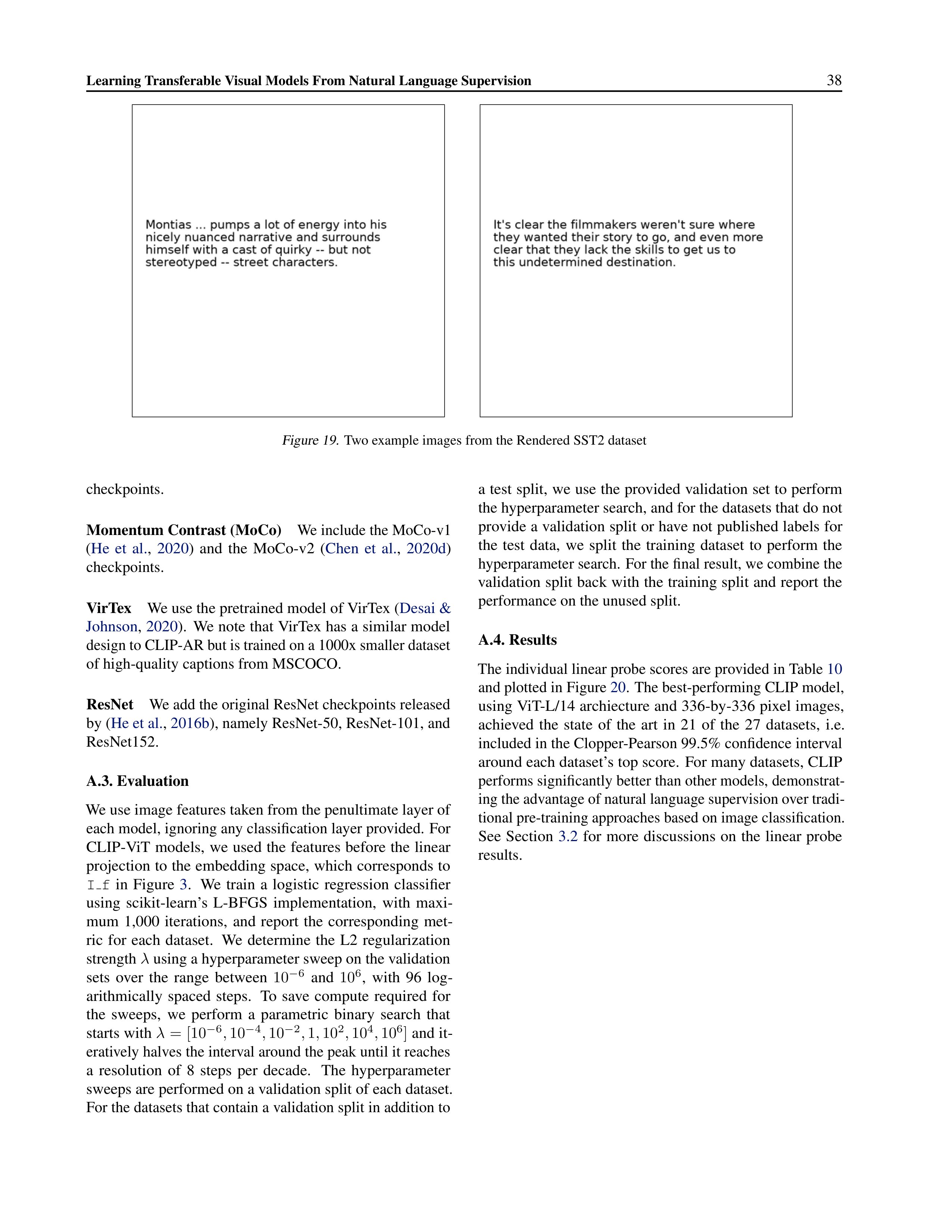
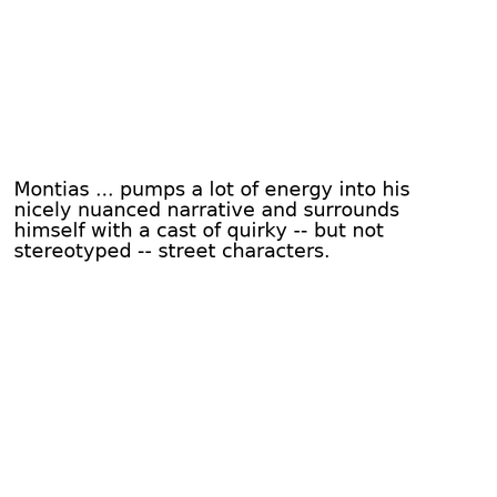
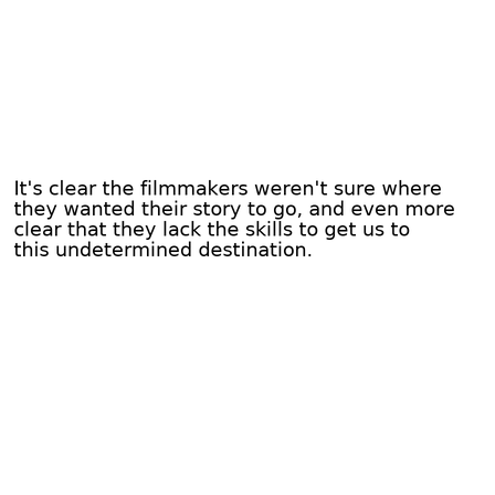
Learning Transferable Visual Models From Natural Language Supervision
38
Figure 19.
Two example images from the Rendered SST2 dataset
checkpoints.
Momentum Contrast (MoCo)
We include the MoCo-v1
(
He
et
al.
,
2020
)
and
the
MoCo-v2
(
Chen
et
al.
,
2020d
)
checkpoints.
VirTex
We use the pretrained model of VirTex (
Desai &
Johnson
,
2020
).
We note that VirTex has a similar model
design to CLIP-AR but is trained on a 1000x smaller dataset
of high-quality captions from MSCOCO.
ResNet
We add the original ResNet checkpoints released
by (
He et al.
,
2016b
), namely ResNet-50, ResNet-101, and
ResNet152.
A.3. Evaluation
We use image features taken from the penultimate layer of
each model, ignoring any classification layer provided.
For
CLIP-ViT
models,
we
used
the
features
before
the
linear
projection to the embedding space, which corresponds to
I
f
in
Figure
3
.
We
train
a
logistic
regression
classifier
using
scikit-learn’s
L-BFGS
implementation,
with
maxi-
mum
1,000
iterations,
and
report
the
corresponding
met-
ric
for
each
dataset.
We
determine
the
L2
regularization
strength
λ
using a hyperparameter sweep on the validation
sets
over
the
range
between
10
−
6
and
10
6
,
with
96
log-
arithmically
spaced
steps.
To
save
compute
required
for
the
sweeps,
we
perform
a
parametric
binary
search
that
starts with
λ
=
[10
−
6
,
10
−
4
,
10
−
2
,
1
,
10
2
,
10
4
,
10
6
]
and it-
eratively halves the interval around the peak until it reaches
a
resolution
of
8
steps
per
decade.
The
hyperparameter
sweeps are performed on a validation split of each dataset.
For the datasets that contain a validation split in addition to
a test split, we use the provided validation set to perform
the hyperparameter search, and for the datasets that do not
provide a validation split or have not published labels for
the
test
data,
we
split
the
training
dataset
to
perform
the
hyperparameter search.
For the final result, we combine the
validation split back with the training split and report the
performance on the unused split.
A.4. Results
The individual linear probe scores are provided in Table
10
and plotted in Figure
20
.
The best-performing CLIP model,
using ViT-L/14 archiecture and 336-by-336 pixel images,
achieved
the
state
of
the
art
in
21
of
the
27
datasets,
i.e.
included in the Clopper-Pearson 99.5% confidence interval
around each dataset’s top score.
For many datasets, CLIP
performs significantly better than other models, demonstrat-
ing the advantage of natural language supervision over tradi-
tional pre-training approaches based on image classification.
See
Section
3.2
for
more
discussions
on
the
linear
probe
results.
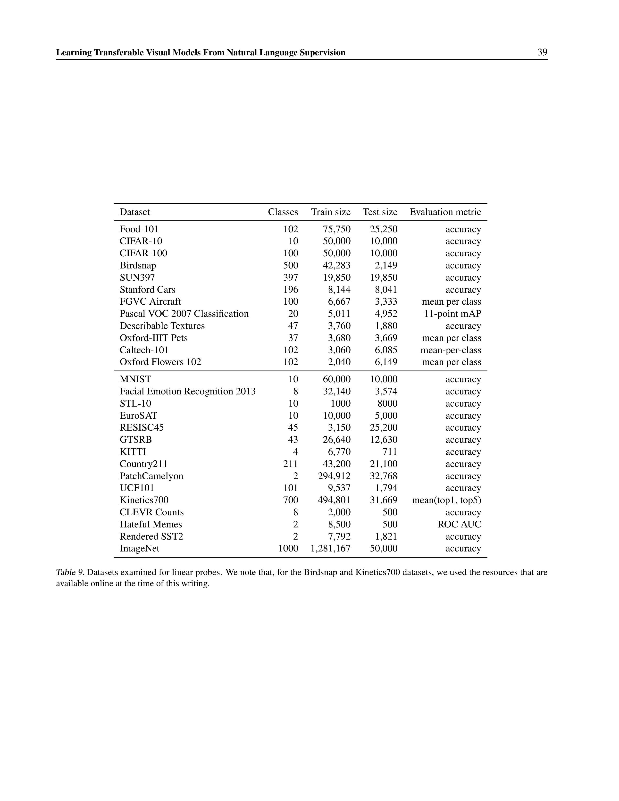
Learning Transferable Visual Models From Natural Language Supervision
39
Dataset
Classes
Train size
Test size
Evaluation metric
Food-101
102
75,750
25,250
accuracy
CIFAR-10
10
50,000
10,000
accuracy
CIFAR-100
100
50,000
10,000
accuracy
Birdsnap
500
42,283
2,149
accuracy
SUN397
397
19,850
19,850
accuracy
Stanford Cars
196
8,144
8,041
accuracy
FGVC Aircraft
100
6,667
3,333
mean per class
Pascal VOC 2007 Classification
20
5,011
4,952
11-point mAP
Describable Textures
47
3,760
1,880
accuracy
Oxford-IIIT Pets
37
3,680
3,669
mean per class
Caltech-101
102
3,060
6,085
mean-per-class
Oxford Flowers 102
102
2,040
6,149
mean per class
MNIST
10
60,000
10,000
accuracy
Facial Emotion Recognition 2013
8
32,140
3,574
accuracy
STL-10
10
1000
8000
accuracy
EuroSAT
10
10,000
5,000
accuracy
RESISC45
45
3,150
25,200
accuracy
GTSRB
43
26,640
12,630
accuracy
KITTI
4
6,770
711
accuracy
Country211
211
43,200
21,100
accuracy
PatchCamelyon
2
294,912
32,768
accuracy
UCF101
101
9,537
1,794
accuracy
Kinetics700
700
494,801
31,669
mean(top1, top5)
CLEVR Counts
8
2,000
500
accuracy
Hateful Memes
2
8,500
500
ROC AUC
Rendered SST2
2
7,792
1,821
accuracy
ImageNet
1000
1,281,167
50,000
accuracy
Table 9.
Datasets examined for linear probes.
We note that, for the Birdsnap and Kinetics700 datasets, we used the resources that are
available online at the time of this writing.
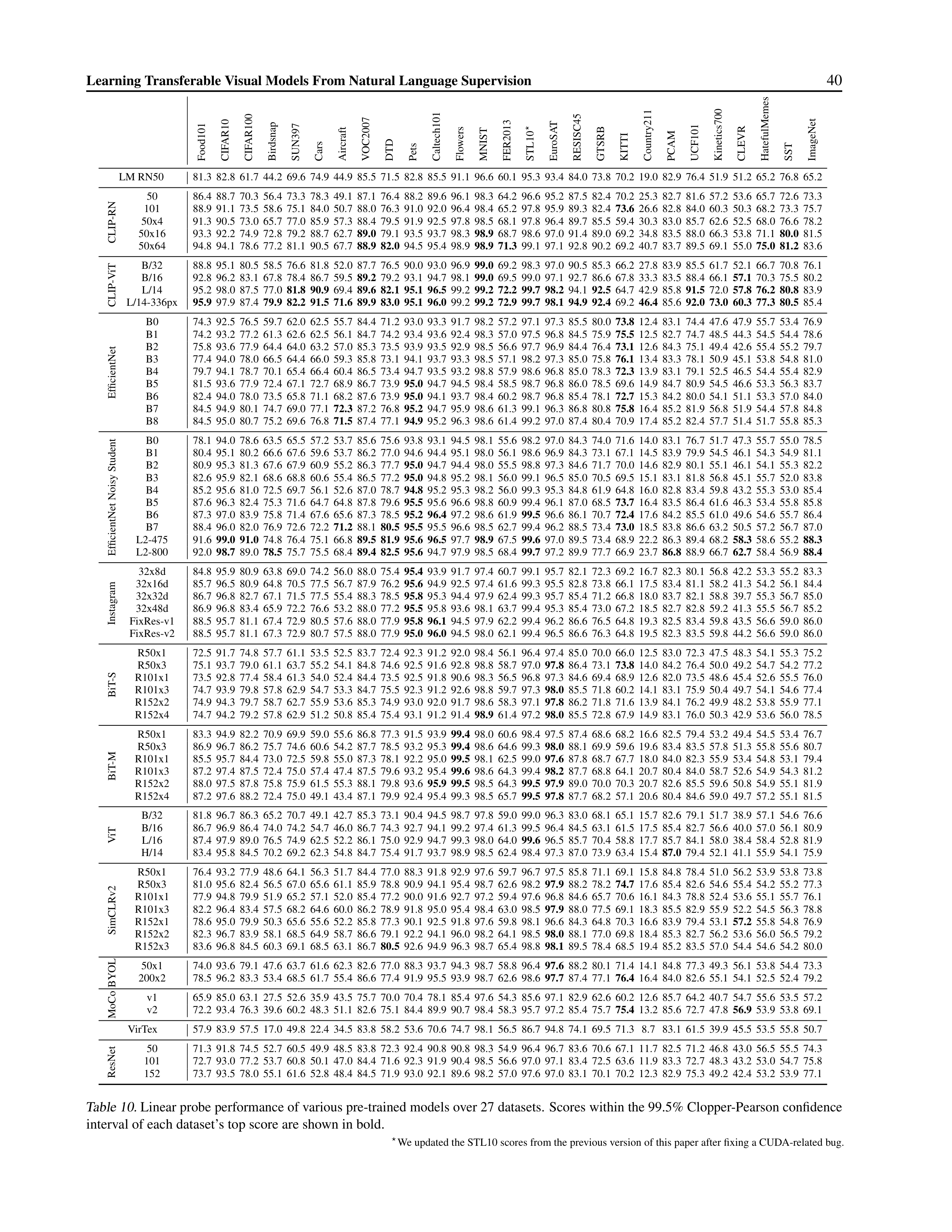
Learning Transferable Visual Models From Natural Language Supervision
40
Food101
CIFAR10
CIFAR100
Birdsnap
SUN397
Cars
Aircraft
VOC2007
DTD
Pets
Caltech101
Flowers
MNIST
FER2013
STL10
⋆
EuroSAT
RESISC45
GTSRB
KITTI
Country211
PCAM
UCF101
Kinetics700
CLEVR
HatefulMemes
SST
ImageNet
LM RN50
81.3
82.8
61.7
44.2
69.6
74.9
44.9
85.5
71.5
82.8
85.5
91.1
96.6
60.1
95.3
93.4
84.0
73.8
70.2
19.0
82.9
76.4
51.9
51.2
65.2
76.8
65.2
CLIP-RN
50
86.4
88.7
70.3
56.4
73.3
78.3
49.1
87.1
76.4
88.2
89.6
96.1
98.3
64.2
96.6
95.2
87.5
82.4
70.2
25.3
82.7
81.6
57.2
53.6
65.7
72.6
73.3
101
88.9
91.1
73.5
58.6
75.1
84.0
50.7
88.0
76.3
91.0
92.0
96.4
98.4
65.2
97.8
95.9
89.3
82.4
73.6
26.6
82.8
84.0
60.3
50.3
68.2
73.3
75.7
50x4
91.3
90.5
73.0
65.7
77.0
85.9
57.3
88.4
79.5
91.9
92.5
97.8
98.5
68.1
97.8
96.4
89.7
85.5
59.4
30.3
83.0
85.7
62.6
52.5
68.0
76.6
78.2
50x16
93.3
92.2
74.9
72.8
79.2
88.7
62.7
89.0
79.1
93.5
93.7
98.3
98.9
68.7
98.6
97.0
91.4
89.0
69.2
34.8
83.5
88.0
66.3
53.8
71.1
80.0
81.5
50x64
94.8
94.1
78.6
77.2
81.1
90.5
67.7
88.9
82.0
94.5
95.4
98.9
98.9
71.3
99.1
97.1
92.8
90.2
69.2
40.7
83.7
89.5
69.1
55.0
75.0
81.2
83.6
CLIP-ViT
B/32
88.8
95.1
80.5
58.5
76.6
81.8
52.0
87.7
76.5
90.0
93.0
96.9
99.0
69.2
98.3
97.0
90.5
85.3
66.2
27.8
83.9
85.5
61.7
52.1
66.7
70.8
76.1
B/16
92.8
96.2
83.1
67.8
78.4
86.7
59.5
89.2
79.2
93.1
94.7
98.1
99.0
69.5
99.0
97.1
92.7
86.6
67.8
33.3
83.5
88.4
66.1
57.1
70.3
75.5
80.2
L/14
95.2
98.0
87.5
77.0
81.8
90.9
69.4
89.6
82.1
95.1
96.5
99.2
99.2
72.2
99.7
98.2
94.1
92.5
64.7
42.9
85.8
91.5
72.0
57.8
76.2
80.8
83.9
L/14-336px
95.9
97.9
87.4
79.9
82.2
91.5
71.6
89.9
83.0
95.1
96.0
99.2
99.2
72.9
99.7
98.1
94.9
92.4
69.2
46.4
85.6
92.0
73.0
60.3
77.3
80.5
85.4
EfficientNet
B0
74.3
92.5
76.5
59.7
62.0
62.5
55.7
84.4
71.2
93.0
93.3
91.7
98.2
57.2
97.1
97.3
85.5
80.0
73.8
12.4
83.1
74.4
47.6
47.9
55.7
53.4
76.9
B1
74.2
93.2
77.2
61.3
62.6
62.5
56.1
84.7
74.2
93.4
93.6
92.4
98.3
57.0
97.5
96.8
84.5
75.9
75.5
12.5
82.7
74.7
48.5
44.3
54.5
54.4
78.6
B2
75.8
93.6
77.9
64.4
64.0
63.2
57.0
85.3
73.5
93.9
93.5
92.9
98.5
56.6
97.7
96.9
84.4
76.4
73.1
12.6
84.3
75.1
49.4
42.6
55.4
55.2
79.7
B3
77.4
94.0
78.0
66.5
64.4
66.0
59.3
85.8
73.1
94.1
93.7
93.3
98.5
57.1
98.2
97.3
85.0
75.8
76.1
13.4
83.3
78.1
50.9
45.1
53.8
54.8
81.0
B4
79.7
94.1
78.7
70.1
65.4
66.4
60.4
86.5
73.4
94.7
93.5
93.2
98.8
57.9
98.6
96.8
85.0
78.3
72.3
13.9
83.1
79.1
52.5
46.5
54.4
55.4
82.9
B5
81.5
93.6
77.9
72.4
67.1
72.7
68.9
86.7
73.9
95.0
94.7
94.5
98.4
58.5
98.7
96.8
86.0
78.5
69.6
14.9
84.7
80.9
54.5
46.6
53.3
56.3
83.7
B6
82.4
94.0
78.0
73.5
65.8
71.1
68.2
87.6
73.9
95.0
94.1
93.7
98.4
60.2
98.7
96.8
85.4
78.1
72.7
15.3
84.2
80.0
54.1
51.1
53.3
57.0
84.0
B7
84.5
94.9
80.1
74.7
69.0
77.1
72.3
87.2
76.8
95.2
94.7
95.9
98.6
61.3
99.1
96.3
86.8
80.8
75.8
16.4
85.2
81.9
56.8
51.9
54.4
57.8
84.8
B8
84.5
95.0
80.7
75.2
69.6
76.8
71.5
87.4
77.1
94.9
95.2
96.3
98.6
61.4
99.2
97.0
87.4
80.4
70.9
17.4
85.2
82.4
57.7
51.4
51.7
55.8
85.3
EfficientNet Noisy Student
B0
78.1
94.0
78.6
63.5
65.5
57.2
53.7
85.6
75.6
93.8
93.1
94.5
98.1
55.6
98.2
97.0
84.3
74.0
71.6
14.0
83.1
76.7
51.7
47.3
55.7
55.0
78.5
B1
80.4
95.1
80.2
66.6
67.6
59.6
53.7
86.2
77.0
94.6
94.4
95.1
98.0
56.1
98.6
96.9
84.3
73.1
67.1
14.5
83.9
79.9
54.5
46.1
54.3
54.9
81.1
B2
80.9
95.3
81.3
67.6
67.9
60.9
55.2
86.3
77.7
95.0
94.7
94.4
98.0
55.5
98.8
97.3
84.6
71.7
70.0
14.6
82.9
80.1
55.1
46.1
54.1
55.3
82.2
B3
82.6
95.9
82.1
68.6
68.8
60.6
55.4
86.5
77.2
95.0
94.8
95.2
98.1
56.0
99.1
96.5
85.0
70.5
69.5
15.1
83.1
81.8
56.8
45.1
55.7
52.0
83.8
B4
85.2
95.6
81.0
72.5
69.7
56.1
52.6
87.0
78.7
94.8
95.2
95.3
98.2
56.0
99.3
95.3
84.8
61.9
64.8
16.0
82.8
83.4
59.8
43.2
55.3
53.0
85.4
B5
87.6
96.3
82.4
75.3
71.6
64.7
64.8
87.8
79.6
95.5
95.6
96.6
98.8
60.9
99.4
96.1
87.0
68.5
73.7
16.4
83.5
86.4
61.6
46.3
53.4
55.8
85.8
B6
87.3
97.0
83.9
75.8
71.4
67.6
65.6
87.3
78.5
95.2
96.4
97.2
98.6
61.9
99.5
96.6
86.1
70.7
72.4
17.6
84.2
85.5
61.0
49.6
54.6
55.7
86.4
B7
88.4
96.0
82.0
76.9
72.6
72.2
71.2
88.1
80.5
95.5
95.5
96.6
98.5
62.7
99.4
96.2
88.5
73.4
73.0
18.5
83.8
86.6
63.2
50.5
57.2
56.7
87.0
L2-475
91.6
99.0
91.0
74.8
76.4
75.1
66.8
89.5
81.9
95.6
96.5
97.7
98.9
67.5
99.6
97.0
89.5
73.4
68.9
22.2
86.3
89.4
68.2
58.3
58.6
55.2
88.3
L2-800
92.0
98.7
89.0
78.5
75.7
75.5
68.4
89.4
82.5
95.6
94.7
97.9
98.5
68.4
99.7
97.2
89.9
77.7
66.9
23.7
86.8
88.9
66.7
62.7
58.4
56.9
88.4
Instagram
32x8d
84.8
95.9
80.9
63.8
69.0
74.2
56.0
88.0
75.4
95.4
93.9
91.7
97.4
60.7
99.1
95.7
82.1
72.3
69.2
16.7
82.3
80.1
56.8
42.2
53.3
55.2
83.3
32x16d
85.7
96.5
80.9
64.8
70.5
77.5
56.7
87.9
76.2
95.6
94.9
92.5
97.4
61.6
99.3
95.5
82.8
73.8
66.1
17.5
83.4
81.1
58.2
41.3
54.2
56.1
84.4
32x32d
86.7
96.8
82.7
67.1
71.5
77.5
55.4
88.3
78.5
95.8
95.3
94.4
97.9
62.4
99.3
95.7
85.4
71.2
66.8
18.0
83.7
82.1
58.8
39.7
55.3
56.7
85.0
32x48d
86.9
96.8
83.4
65.9
72.2
76.6
53.2
88.0
77.2
95.5
95.8
93.6
98.1
63.7
99.4
95.3
85.4
73.0
67.2
18.5
82.7
82.8
59.2
41.3
55.5
56.7
85.2
FixRes-v1
88.5
95.7
81.1
67.4
72.9
80.5
57.6
88.0
77.9
95.8
96.1
94.5
97.9
62.2
99.4
96.2
86.6
76.5
64.8
19.3
82.5
83.4
59.8
43.5
56.6
59.0
86.0
FixRes-v2
88.5
95.7
81.1
67.3
72.9
80.7
57.5
88.0
77.9
95.0
96.0
94.5
98.0
62.1
99.4
96.5
86.6
76.3
64.8
19.5
82.3
83.5
59.8
44.2
56.6
59.0
86.0
BiT-S
R50x1
72.5
91.7
74.8
57.7
61.1
53.5
52.5
83.7
72.4
92.3
91.2
92.0
98.4
56.1
96.4
97.4
85.0
70.0
66.0
12.5
83.0
72.3
47.5
48.3
54.1
55.3
75.2
R50x3
75.1
93.7
79.0
61.1
63.7
55.2
54.1
84.8
74.6
92.5
91.6
92.8
98.8
58.7
97.0
97.8
86.4
73.1
73.8
14.0
84.2
76.4
50.0
49.2
54.7
54.2
77.2
R101x1
73.5
92.8
77.4
58.4
61.3
54.0
52.4
84.4
73.5
92.5
91.8
90.6
98.3
56.5
96.8
97.3
84.6
69.4
68.9
12.6
82.0
73.5
48.6
45.4
52.6
55.5
76.0
R101x3
74.7
93.9
79.8
57.8
62.9
54.7
53.3
84.7
75.5
92.3
91.2
92.6
98.8
59.7
97.3
98.0
85.5
71.8
60.2
14.1
83.1
75.9
50.4
49.7
54.1
54.6
77.4
R152x2
74.9
94.3
79.7
58.7
62.7
55.9
53.6
85.3
74.9
93.0
92.0
91.7
98.6
58.3
97.1
97.8
86.2
71.8
71.6
13.9
84.1
76.2
49.9
48.2
53.8
55.9
77.1
R152x4
74.7
94.2
79.2
57.8
62.9
51.2
50.8
85.4
75.4
93.1
91.2
91.4
98.9
61.4
97.2
98.0
85.5
72.8
67.9
14.9
83.1
76.0
50.3
42.9
53.6
56.0
78.5
BiT-M
R50x1
83.3
94.9
82.2
70.9
69.9
59.0
55.6
86.8
77.3
91.5
93.9
99.4
98.0
60.6
98.4
97.5
87.4
68.6
68.2
16.6
82.5
79.4
53.2
49.4
54.5
53.4
76.7
R50x3
86.9
96.7
86.2
75.7
74.6
60.6
54.2
87.7
78.5
93.2
95.3
99.4
98.6
64.6
99.3
98.0
88.1
69.9
59.6
19.6
83.4
83.5
57.8
51.3
55.8
55.6
80.7
R101x1
85.5
95.7
84.4
73.0
72.5
59.8
55.0
87.3
78.1
92.2
95.0
99.5
98.1
62.5
99.0
97.6
87.8
68.7
67.7
18.0
84.0
82.3
55.9
53.4
54.8
53.1
79.4
R101x3
87.2
97.4
87.5
72.4
75.0
57.4
47.4
87.5
79.6
93.2
95.4
99.6
98.6
64.3
99.4
98.2
87.7
68.8
64.1
20.7
80.4
84.0
58.7
52.6
54.9
54.3
81.2
R152x2
88.0
97.5
87.8
75.8
75.9
61.5
55.3
88.1
79.8
93.6
95.9
99.5
98.5
64.3
99.5
97.9
89.0
70.0
70.3
20.7
82.6
85.5
59.6
50.8
54.9
55.1
81.9
R152x4
87.2
97.6
88.2
72.4
75.0
49.1
43.4
87.1
79.9
92.4
95.4
99.3
98.5
65.7
99.5
97.8
87.7
68.2
57.1
20.6
80.4
84.6
59.0
49.7
57.2
55.1
81.5
ViT
B/32
81.8
96.7
86.3
65.2
70.7
49.1
42.7
85.3
73.1
90.4
94.5
98.7
97.8
59.0
99.0
96.3
83.0
68.1
65.1
15.7
82.6
79.1
51.7
38.9
57.1
54.6
76.6
B/16
86.7
96.9
86.4
74.0
74.2
54.7
46.0
86.7
74.3
92.7
94.1
99.2
97.4
61.3
99.5
96.4
84.5
63.1
61.5
17.5
85.4
82.7
56.6
40.0
57.0
56.1
80.9
L/16
87.4
97.9
89.0
76.5
74.9
62.5
52.2
86.1
75.0
92.9
94.7
99.3
98.0
64.0
99.6
96.5
85.7
70.4
58.8
17.7
85.7
84.1
58.0
38.4
58.4
52.8
81.9
H/14
83.4
95.8
84.5
70.2
69.2
62.3
54.8
84.7
75.4
91.7
93.7
98.9
98.5
62.4
98.4
97.3
87.0
73.9
63.4
15.4
87.0
79.4
52.1
41.1
55.9
54.1
75.9
SimCLRv2
R50x1
76.4
93.2
77.9
48.6
64.1
56.3
51.7
84.4
77.0
88.3
91.8
92.9
97.6
59.7
96.7
97.5
85.8
71.1
69.1
15.8
84.8
78.4
51.0
56.2
53.9
53.8
73.8
R50x3
81.0
95.6
82.4
56.5
67.0
65.6
61.1
85.9
78.8
90.9
94.1
95.4
98.7
62.6
98.2
97.9
88.2
78.2
74.7
17.6
85.4
82.6
54.6
55.4
54.2
55.2
77.3
R101x1
77.9
94.8
79.9
51.9
65.2
57.1
52.0
85.4
77.2
90.0
91.6
92.7
97.2
59.4
97.6
96.8
84.6
65.7
70.6
16.1
84.3
78.8
52.4
53.6
55.1
55.7
76.1
R101x3
82.2
96.4
83.4
57.5
68.2
64.6
60.0
86.2
78.9
91.8
95.0
95.4
98.4
63.0
98.5
97.9
88.0
77.5
69.1
18.3
85.5
82.9
55.9
52.2
54.5
56.3
78.8
R152x1
78.6
95.0
79.9
50.3
65.6
55.6
52.2
85.8
77.3
90.1
92.5
91.8
97.6
59.8
98.1
96.6
84.3
64.8
70.3
16.6
83.9
79.4
53.1
57.2
55.8
54.8
76.9
R152x2
82.3
96.7
83.9
58.1
68.5
64.9
58.7
86.6
79.1
92.2
94.1
96.0
98.2
64.1
98.5
98.0
88.1
77.0
69.8
18.4
85.3
82.7
56.2
53.6
56.0
56.5
79.2
R152x3
83.6
96.8
84.5
60.3
69.1
68.5
63.1
86.7
80.5
92.6
94.9
96.3
98.7
65.4
98.8
98.1
89.5
78.4
68.5
19.4
85.2
83.5
57.0
54.4
54.6
54.2
80.0
BYOL
50x1
74.0
93.6
79.1
47.6
63.7
61.6
62.3
82.6
77.0
88.3
93.7
94.3
98.7
58.8
96.4
97.6
88.2
80.1
71.4
14.1
84.8
77.3
49.3
56.1
53.8
54.4
73.3
200x2
78.5
96.2
83.3
53.4
68.5
61.7
55.4
86.6
77.4
91.9
95.5
93.9
98.7
62.6
98.6
97.7
87.4
77.1
76.4
16.4
84.0
82.6
55.1
54.1
52.5
52.4
79.2
MoCo
v1
65.9
85.0
63.1
27.5
52.6
35.9
43.5
75.7
70.0
70.4
78.1
85.4
97.6
54.3
85.6
97.1
82.9
62.6
60.2
12.6
85.7
64.2
40.7
54.7
55.6
53.5
57.2
v2
72.2
93.4
76.3
39.6
60.2
48.3
51.1
82.6
75.1
84.4
89.9
90.7
98.4
58.3
95.7
97.2
85.4
75.7
75.4
13.2
85.6
72.7
47.8
56.9
53.9
53.8
69.1
VirTex
57.9
83.9
57.5
17.0
49.8
22.4
34.5
83.8
58.2
53.6
70.6
74.7
98.1
56.5
86.7
94.8
74.1
69.5
71.3
8.7
83.1
61.5
39.9
45.5
53.5
55.8
50.7
ResNet
50
71.3
91.8
74.5
52.7
60.5
49.9
48.5
83.8
72.3
92.4
90.8
90.8
98.3
54.9
96.4
96.7
83.6
70.6
67.1
11.7
82.5
71.2
46.8
43.0
56.5
55.5
74.3
101
72.7
93.0
77.2
53.7
60.8
50.1
47.0
84.4
71.6
92.3
91.9
90.4
98.5
56.6
97.0
97.1
83.4
72.5
63.6
11.9
83.3
72.7
48.3
43.2
53.0
54.7
75.8
152
73.7
93.5
78.0
55.1
61.6
52.8
48.4
84.5
71.9
93.0
92.1
89.6
98.2
57.0
97.6
97.0
83.1
70.1
70.2
12.3
82.9
75.3
49.2
42.4
53.2
53.9
77.1
Table 10.
Linear probe performance of various pre-trained models over 27 datasets.
Scores within the 99.5% Clopper-Pearson confidence
interval of each dataset’s top score are shown in bold.
⋆
We updated the STL10 scores from the previous version of this paper after fixing a CUDA-related bug.
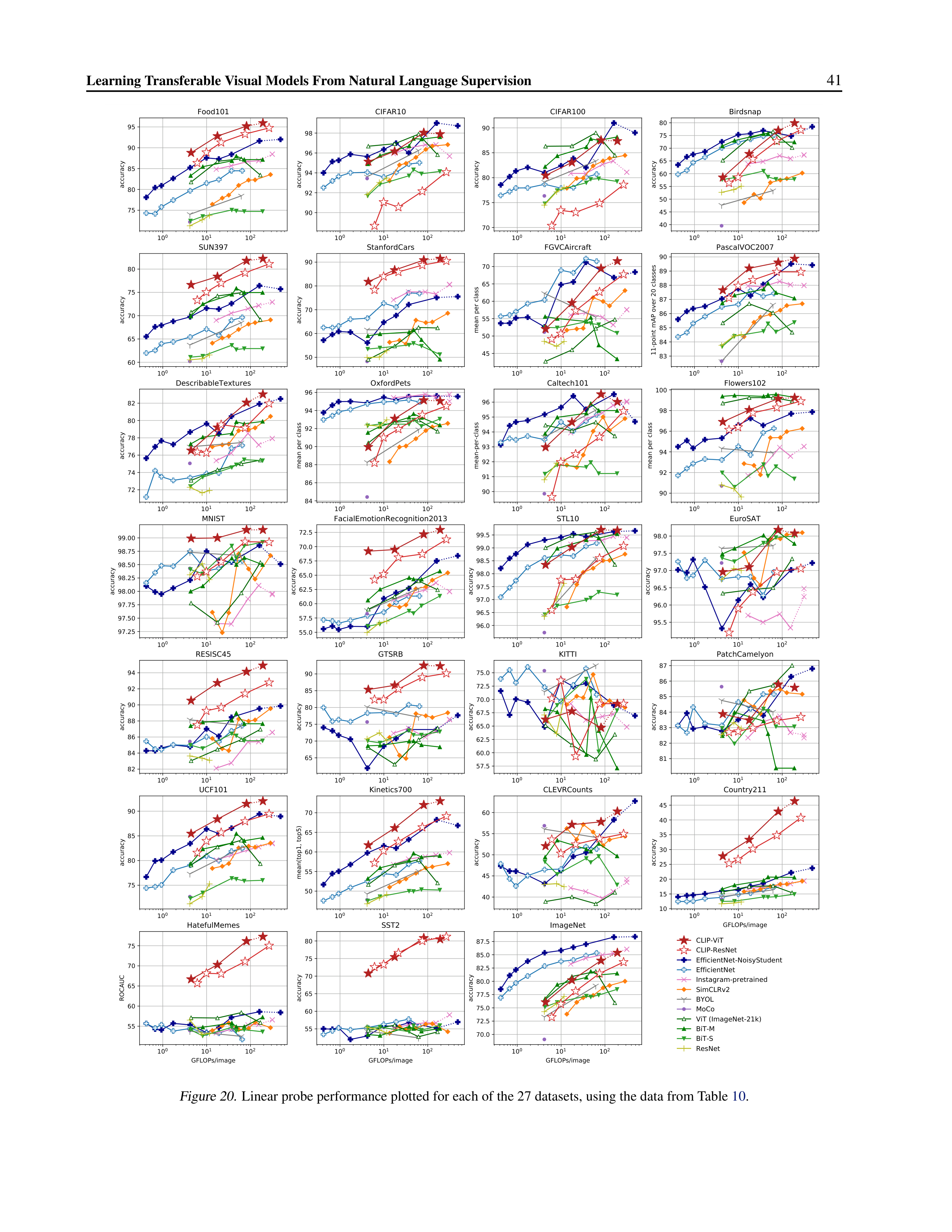
Learning Transferable Visual Models From Natural Language Supervision
41
10
0
10
1
10
2
75
80
85
90
95
accuracy
Food101
10
0
10
1
10
2
90
92
94
96
98
accuracy
CIFAR10
10
0
10
1
10
2
70
75
80
85
90
accuracy
CIFAR100
10
0
10
1
10
2
40
45
50
55
60
65
70
75
80
accuracy
Birdsnap
10
0
10
1
10
2
60
65
70
75
80
accuracy
SUN397
10
0
10
1
10
2
50
60
70
80
90
accuracy
StanfordCars
10
0
10
1
10
2
45
50
55
60
65
70
mean per class
FGVCAircraft
10
0
10
1
10
2
83
84
85
86
87
88
89
90
11-point mAP over 20 classes
PascalVOC2007
10
0
10
1
10
2
72
74
76
78
80
82
accuracy
DescribableTextures
10
0
10
1
10
2
84
86
88
90
92
94
96
mean per class
OxfordPets
10
0
10
1
10
2
90
91
92
93
94
95
96
mean-per-class
Caltech101
10
0
10
1
10
2
90
92
94
96
98
100
mean per class
Flowers102
10
0
10
1
10
2
97.25
97.50
97.75
98.00
98.25
98.50
98.75
99.00
accuracy
MNIST
10
0
10
1
10
2
55.0
57.5
60.0
62.5
65.0
67.5
70.0
72.5
accuracy
FacialEmotionRecognition2013
10
0
10
1
10
2
96.0
96.5
97.0
97.5
98.0
98.5
99.0
99.5
accuracy
STL10
10
0
10
1
10
2
95.5
96.0
96.5
97.0
97.5
98.0
accuracy
EuroSAT
10
0
10
1
10
2
82
84
86
88
90
92
94
accuracy
RESISC45
10
0
10
1
10
2
65
70
75
80
85
90
accuracy
GTSRB
10
0
10
1
10
2
57.5
60.0
62.5
65.0
67.5
70.0
72.5
75.0
accuracy
KITTI
10
0
10
1
10
2
81
82
83
84
85
86
87
accuracy
PatchCamelyon
10
0
10
1
10
2
75
80
85
90
accuracy
UCF101
10
0
10
1
10
2
50
55
60
65
70
mean(top1, top5)
Kinetics700
10
0
10
1
10
2
40
45
50
55
60
accuracy
CLEVRCounts
10
0
10
1
10
2
GFLOPs/image
10
15
20
25
30
35
40
45
accuracy
Country211
10
0
10
1
10
2
GFLOPs/image
55
60
65
70
75
ROCAUC
HatefulMemes
10
0
10
1
10
2
GFLOPs/image
55
60
65
70
75
80
accuracy
SST2
10
0
10
1
10
2
GFLOPs/image
70.0
72.5
75.0
77.5
80.0
82.5
85.0
87.5
accuracy
ImageNet
CLIP-ViT
CLIP-ResNet
EfficientNet-NoisyStudent
EfficientNet
Instagram-pretrained
SimCLRv2
BYOL
MoCo
ViT (ImageNet-21k)
BiT-M
BiT-S
ResNet
Figure 20.
Linear probe performance plotted for each of the 27 datasets, using the data from Table
10
.
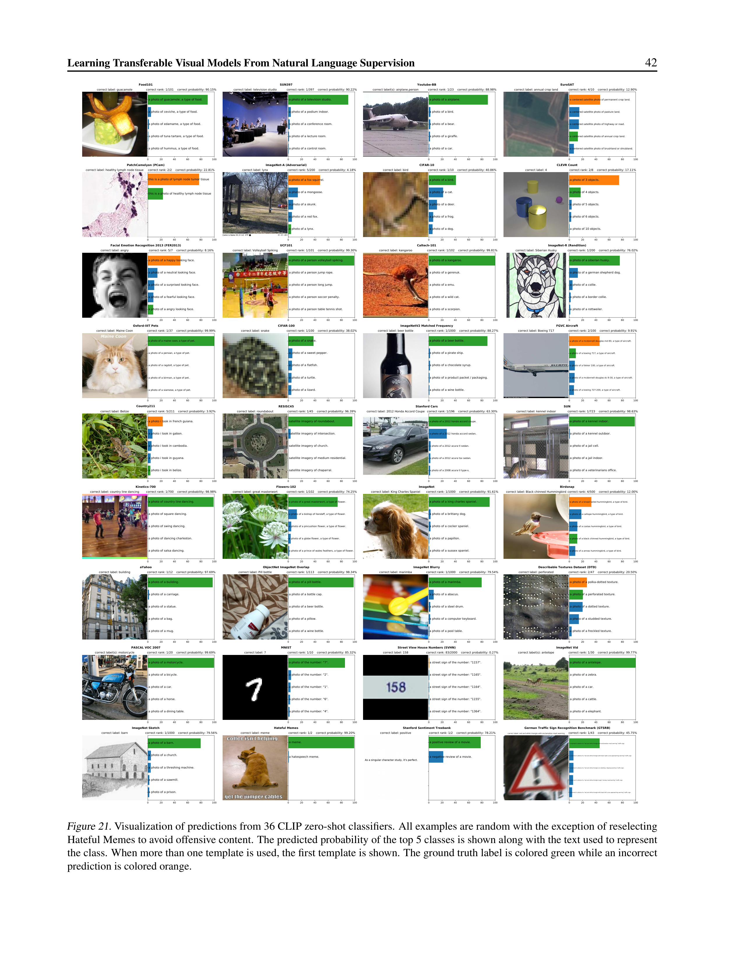





Learning Transferable Visual Models From Natural Language Supervision
42
correct label: red and white triangle with exclamation mark warning
0
20
40
60
80
100
a zoomed in photo of a "red and white triangle with exclamation mark warning" traffic sign.
a zoomed in photo of a "red and white triangle with black right curve approaching warning" traffic sign.
a zoomed in photo of a "red and white triangle car skidding / slipping warning" traffic sign.
a zoomed in photo of a "red and white triangle rough / bumpy road warning" traffic sign.
a zoomed in photo of a "red and white triangle with black left curve approaching warning" traffic sign.
correct rank: 1/43 correct probability: 45.75%
German Traffic Sign Recognition Benchmark (GTSRB)
correct label: positive
0
20
40
60
80
100
a positive review of a movie.
a negative review of a movie.
correct rank: 1/2 correct probability: 78.21%
Stanford Sentiment Treebank
correct label: meme
0
20
40
60
80
100
a meme.
a hatespeech meme.
correct rank: 1/2 correct probability: 99.20%
Hateful Memes
correct label: barn
0
20
40
60
80
100
a photo of a barn.
a photo of a church.
a photo of a threshing machine.
a photo of a sawmill.
a photo of a prison.
correct rank: 1/1000 correct probability: 79.56%
ImageNet Sketch
correct label(s): antelope
0
20
40
60
80
100
a photo of a antelope.
a photo of a zebra.
a photo of a car.
a photo of a cattle.
a photo of a elephant.
correct rank: 1/30 correct probability: 99.77%
ImageNet Vid
correct label: 158
0
20
40
60
80
100
a street sign of the number: "1157".
a street sign of the number: "1165".
a street sign of the number: "1164".
a street sign of the number: "1155".
a street sign of the number: "1364".
correct rank: 83/2000 correct probability: 0.27%
Street View House Numbers (SVHN)
correct label: 7
0
20
40
60
80
100
a photo of the number: "7".
a photo of the number: "2".
a photo of the number: "1".
a photo of the number: "6".
a photo of the number: "4".
correct rank: 1/10 correct probability: 85.32%
MNIST
correct label(s): motorcycle
0
20
40
60
80
100
a photo of a motorcycle.
a photo of a bicycle.
a photo of a car.
a photo of a horse.
a photo of a dining table.
correct rank: 1/20 correct probability: 99.69%
PASCAL VOC 2007
correct label: perforated
0
20
40
60
80
100
a photo of a polka-dotted texture.
a photo of a perforated texture.
a photo of a dotted texture.
a photo of a studded texture.
a photo of a freckled texture.
correct rank: 2/47 correct probability: 20.50%
Describable Textures Dataset (DTD)
correct label: marimba
0
20
40
60
80
100
a photo of a marimba.
a photo of a abacus.
a photo of a steel drum.
a photo of a computer keyboard.
a photo of a pool table.
correct rank: 1/1000 correct probability: 79.54%
ImageNet Blurry
correct label: Pill bottle
0
20
40
60
80
100
a photo of a pill bottle.
a photo of a bottle cap.
a photo of a beer bottle.
a photo of a pillow.
a photo of a wine bottle.
correct rank: 1/113 correct probability: 98.34%
ObjectNet ImageNet Overlap
correct label: building
0
20
40
60
80
100
a photo of a building.
a photo of a carriage.
a photo of a statue.
a photo of a bag.
a photo of a mug.
correct rank: 1/12 correct probability: 97.69%
aYahoo
correct label: Black chinned Hummingbird
0
20
40
60
80
100
a photo of a broad tailed hummingbird, a type of bird.
a photo of a calliope hummingbird, a type of bird.
a photo of a costas hummingbird, a type of bird.
a photo of a black chinned hummingbird, a type of bird.
a photo of a annas hummingbird, a type of bird.
correct rank: 4/500 correct probability: 12.00%
Birdsnap
correct label: King Charles Spaniel
0
20
40
60
80
100
a photo of a king charles spaniel.
a photo of a brittany dog.
a photo of a cocker spaniel.
a photo of a papillon.
a photo of a sussex spaniel.
correct rank: 1/1000 correct probability: 91.61%
ImageNet
correct label: great masterwort
0
20
40
60
80
100
a photo of a great masterwort, a type of flower.
a photo of a bishop of llandaff, a type of flower.
a photo of a pincushion flower, a type of flower.
a photo of a globe flower, a type of flower.
a photo of a prince of wales feathers, a type of flower.
correct rank: 1/102 correct probability: 74.25%
Flowers-102
correct label: country line dancing
0
20
40
60
80
100
a photo of country line dancing.
a photo of square dancing.
a photo of swing dancing.
a photo of dancing charleston.
a photo of salsa dancing.
correct rank: 1/700 correct probability: 98.98%
Kinetics-700
correct label: kennel indoor
0
20
40
60
80
100
a photo of a kennel indoor.
a photo of a kennel outdoor.
a photo of a jail cell.
a photo of a jail indoor.
a photo of a veterinarians office.
correct rank: 1/723 correct probability: 98.63%
SUN
correct label: 2012 Honda Accord Coupe
0
20
40
60
80
100
a photo of a 2012 honda accord coupe.
a photo of a 2012 honda accord sedan.
a photo of a 2012 acura tl sedan.
a photo of a 2012 acura tsx sedan.
a photo of a 2008 acura tl type-s.
correct rank: 1/196 correct probability: 63.30%
Stanford Cars
correct label: roundabout
0
20
40
60
80
100
satellite imagery of roundabout.
satellite imagery of intersection.
satellite imagery of church.
satellite imagery of medium residential.
satellite imagery of chaparral.
correct rank: 1/45 correct probability: 96.39%
RESISC45
correct label: Belize
0
20
40
60
80
100
a photo i took in french guiana.
a photo i took in gabon.
a photo i took in cambodia.
a photo i took in guyana.
a photo i took in belize.
correct rank: 5/211 correct probability: 3.92%
Country211
correct label: Boeing 717
0
20
40
60
80
100
a photo of a mcdonnell douglas md-90, a type of aircraft.
a photo of a boeing 717, a type of aircraft.
a photo of a fokker 100, a type of aircraft.
a photo of a mcdonnell douglas dc-9-30, a type of aircraft.
a photo of a boeing 727-200, a type of aircraft.
correct rank: 2/100 correct probability: 9.91%
FGVC Aircraft
correct label: beer bottle
0
20
40
60
80
100
a photo of a beer bottle.
a photo of a pirate ship.
a photo of a chocolate syrup.
a photo of a product packet / packaging.
a photo of a wine bottle.
correct rank: 1/1000 correct probability: 88.27%
ImageNetV2 Matched Frequency
correct label: snake
0
20
40
60
80
100
a photo of a snake.
a photo of a sweet pepper.
a photo of a flatfish.
a photo of a turtle.
a photo of a lizard.
correct rank: 1/100 correct probability: 38.02%
CIFAR-100
correct label: Maine Coon
0
20
40
60
80
100
a photo of a maine coon, a type of pet.
a photo of a persian, a type of pet.
a photo of a ragdoll, a type of pet.
a photo of a birman, a type of pet.
a photo of a siamese, a type of pet.
correct rank: 1/37 correct probability: 99.99%
Oxford-IIIT Pets
correct label: Siberian Husky
0
20
40
60
80
100
a photo of a siberian husky.
a photo of a german shepherd dog.
a photo of a collie.
a photo of a border collie.
a photo of a rottweiler.
correct rank: 1/200 correct probability: 76.02%
ImageNet-R (Rendition)
correct label: kangaroo
0
20
40
60
80
100
a photo of a kangaroo.
a photo of a gerenuk.
a photo of a emu.
a photo of a wild cat.
a photo of a scorpion.
correct rank: 1/102 correct probability: 99.81%
Caltech-101
correct label: Volleyball Spiking
0
20
40
60
80
100
a photo of a person volleyball spiking.
a photo of a person jump rope.
a photo of a person long jump.
a photo of a person soccer penalty.
a photo of a person table tennis shot.
correct rank: 1/101 correct probability: 99.30%
UCF101
correct label: angry
0
20
40
60
80
100
a photo of a happy looking face.
a photo of a neutral looking face.
a photo of a surprised looking face.
a photo of a fearful looking face.
a photo of a angry looking face.
correct rank: 5/7 correct probability: 8.16%
Facial Emotion Recognition 2013 (FER2013)
correct label: 4
0
20
40
60
80
100
a photo of 3 objects.
a photo of 4 objects.
a photo of 5 objects.
a photo of 6 objects.
a photo of 10 objects.
correct rank: 2/8 correct probability: 17.11%
CLEVR Count
correct label: bird
0
20
40
60
80
100
a photo of a bird.
a photo of a cat.
a photo of a deer.
a photo of a frog.
a photo of a dog.
correct rank: 1/10 correct probability: 40.86%
CIFAR-10
correct label: lynx
0
20
40
60
80
100
a photo of a fox squirrel.
a photo of a mongoose.
a photo of a skunk.
a photo of a red fox.
a photo of a lynx.
correct rank: 5/200 correct probability: 4.18%
ImageNet-A (Adversarial)
correct label: healthy lymph node tissue
0
20
40
60
80
100
this is a photo of lymph node tumor tissue
this is a photo of healthy lymph node tissue
correct rank: 2/2 correct probability: 22.81%
PatchCamelyon (PCam)
correct label: annual crop land
0
20
40
60
80
100
a centered satellite photo of permanent crop land.
a centered satellite photo of pasture land.
a centered satellite photo of highway or road.
a centered satellite photo of annual crop land.
a centered satellite photo of brushland or shrubland.
correct rank: 4/10 correct probability: 12.90%
EuroSAT
correct label(s): airplane,person
0
20
40
60
80
100
a photo of a airplane.
a photo of a bird.
a photo of a bear.
a photo of a giraffe.
a photo of a car.
correct rank: 1/23 correct probability: 88.98%
Youtube-BB
correct label: television studio
0
20
40
60
80
100
a photo of a television studio.
a photo of a podium indoor.
a photo of a conference room.
a photo of a lecture room.
a photo of a control room.
correct rank: 1/397 correct probability: 90.22%
SUN397
correct label: guacamole
0
20
40
60
80
100
a photo of guacamole, a type of food.
a photo of ceviche, a type of food.
a photo of edamame, a type of food.
a photo of tuna tartare, a type of food.
a photo of hummus, a type of food.
correct rank: 1/101 correct probability: 90.15%
Food101
Figure 21.
Visualization of predictions from 36 CLIP zero-shot classifiers.
All examples are random with the exception of reselecting
Hateful Memes to avoid offensive content.
The predicted probability of the top 5 classes is shown along with the text used to represent
the class.
When more than one template is used, the first template is shown.
The ground truth label is colored green while an incorrect
prediction is colored orange.
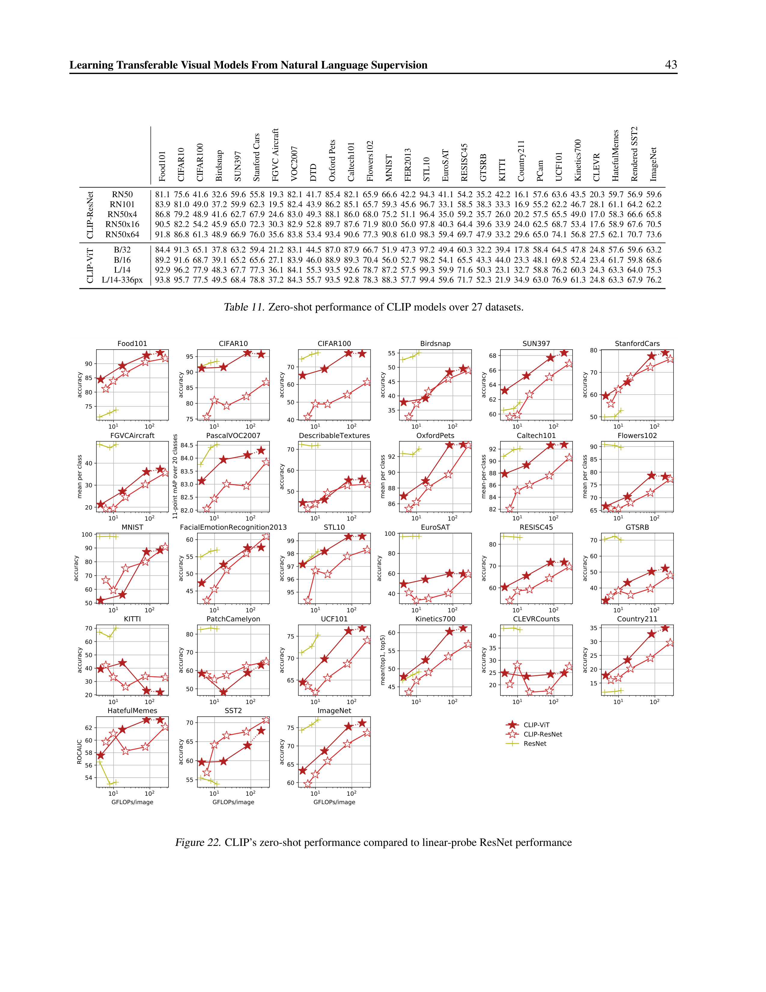
Learning Transferable Visual Models From Natural Language Supervision
43
Food101
CIFAR10
CIFAR100
Birdsnap
SUN397
Stanford Cars
FGVC Aircraft
VOC2007
DTD
Oxford Pets
Caltech101
Flowers102
MNIST
FER2013
STL10
EuroSAT
RESISC45
GTSRB
KITTI
Country211
PCam
UCF101
Kinetics700
CLEVR
HatefulMemes
Rendered SST2
ImageNet
CLIP-ResNet
RN50
81.1
75.6
41.6
32.6
59.6
55.8
19.3
82.1
41.7
85.4
82.1
65.9
66.6
42.2
94.3
41.1
54.2
35.2
42.2
16.1
57.6
63.6
43.5
20.3
59.7
56.9
59.6
RN101
83.9
81.0
49.0
37.2
59.9
62.3
19.5
82.4
43.9
86.2
85.1
65.7
59.3
45.6
96.7
33.1
58.5
38.3
33.3
16.9
55.2
62.2
46.7
28.1
61.1
64.2
62.2
RN50x4
86.8
79.2
48.9
41.6
62.7
67.9
24.6
83.0
49.3
88.1
86.0
68.0
75.2
51.1
96.4
35.0
59.2
35.7
26.0
20.2
57.5
65.5
49.0
17.0
58.3
66.6
65.8
RN50x16
90.5
82.2
54.2
45.9
65.0
72.3
30.3
82.9
52.8
89.7
87.6
71.9
80.0
56.0
97.8
40.3
64.4
39.6
33.9
24.0
62.5
68.7
53.4
17.6
58.9
67.6
70.5
RN50x64
91.8
86.8
61.3
48.9
66.9
76.0
35.6
83.8
53.4
93.4
90.6
77.3
90.8
61.0
98.3
59.4
69.7
47.9
33.2
29.6
65.0
74.1
56.8
27.5
62.1
70.7
73.6
CLIP-ViT
B/32
84.4
91.3
65.1
37.8
63.2
59.4
21.2
83.1
44.5
87.0
87.9
66.7
51.9
47.3
97.2
49.4
60.3
32.2
39.4
17.8
58.4
64.5
47.8
24.8
57.6
59.6
63.2
B/16
89.2
91.6
68.7
39.1
65.2
65.6
27.1
83.9
46.0
88.9
89.3
70.4
56.0
52.7
98.2
54.1
65.5
43.3
44.0
23.3
48.1
69.8
52.4
23.4
61.7
59.8
68.6
L/14
92.9
96.2
77.9
48.3
67.7
77.3
36.1
84.1
55.3
93.5
92.6
78.7
87.2
57.5
99.3
59.9
71.6
50.3
23.1
32.7
58.8
76.2
60.3
24.3
63.3
64.0
75.3
L/14-336px
93.8
95.7
77.5
49.5
68.4
78.8
37.2
84.3
55.7
93.5
92.8
78.3
88.3
57.7
99.4
59.6
71.7
52.3
21.9
34.9
63.0
76.9
61.3
24.8
63.3
67.9
76.2
Table 11.
Zero-shot performance of CLIP models over 27 datasets.
10
1
10
2
75
80
85
90
accuracy
Food101
10
1
10
2
75
80
85
90
95
accuracy
CIFAR10
10
1
10
2
40
50
60
70
accuracy
CIFAR100
10
1
10
2
35
40
45
50
55
accuracy
Birdsnap
10
1
10
2
60
62
64
66
68
accuracy
SUN397
10
1
10
2
50
60
70
80
accuracy
StanfordCars
10
1
10
2
20
30
40
mean per class
FGVCAircraft
10
1
10
2
82.0
82.5
83.0
83.5
84.0
84.5
11-point mAP over 20 classes
PascalVOC2007
10
1
10
2
50
60
70
accuracy
DescribableTextures
10
1
10
2
86
88
90
92
mean per class
OxfordPets
10
1
10
2
82
84
86
88
90
92
mean-per-class
Caltech101
10
1
10
2
65
70
75
80
85
90
mean per class
Flowers102
10
1
10
2
50
60
70
80
90
100
accuracy
MNIST
10
1
10
2
45
50
55
60
accuracy
FacialEmotionRecognition2013
10
1
10
2
95
96
97
98
99
accuracy
STL10
10
1
10
2
40
60
80
100
accuracy
EuroSAT
10
1
10
2
60
70
80
accuracy
RESISC45
10
1
10
2
40
50
60
70
accuracy
GTSRB
10
1
10
2
20
30
40
50
60
70
accuracy
KITTI
10
1
10
2
50
60
70
80
accuracy
PatchCamelyon
10
1
10
2
65
70
75
accuracy
UCF101
10
1
10
2
45
50
55
60
mean(top1, top5)
Kinetics700
10
1
10
2
20
25
30
35
40
accuracy
CLEVRCounts
10
1
10
2
15
20
25
30
35
accuracy
Country211
10
1
10
2
GFLOPs/image
54
56
58
60
62
ROCAUC
HatefulMemes
10
1
10
2
GFLOPs/image
55
60
65
70
accuracy
SST2
10
1
10
2
GFLOPs/image
60
65
70
75
accuracy
ImageNet
CLIP-ViT
CLIP-ResNet
ResNet
Figure 22.
CLIP’s zero-shot performance compared to linear-probe ResNet performance
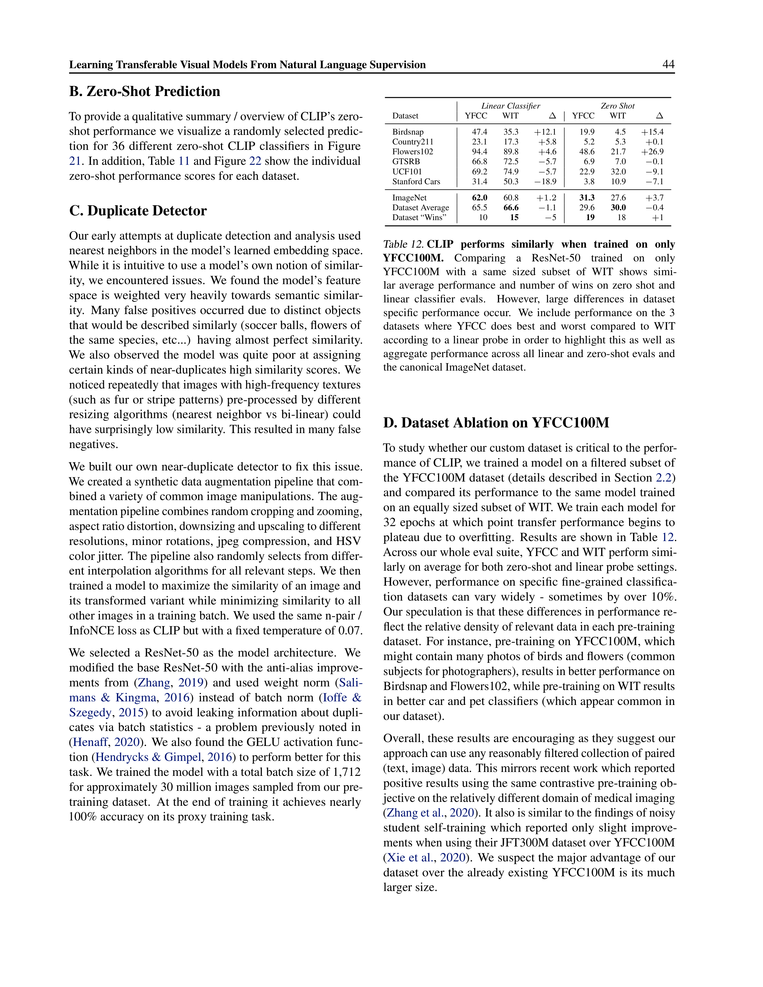
Learning Transferable Visual Models From Natural Language Supervision
44
B. Zero-Shot Prediction
To provide a qualitative summary / overview of CLIP’s zero-
shot performance we visualize a randomly selected predic-
tion
for
36
different
zero-shot
CLIP
classifiers
in
Figure
21
.
In addition, Table
11
and Figure
22
show the individual
zero-shot performance scores for each dataset.
C. Duplicate Detector
Our early attempts at duplicate detection and analysis used
nearest neighbors in the model’s learned embedding space.
While it is intuitive to use a model’s own notion of similar-
ity, we encountered issues.
We found the model’s feature
space
is
weighted
very
heavily
towards
semantic
similar-
ity.
Many
false
positives
occurred
due
to
distinct
objects
that would be described similarly (soccer balls, flowers of
the
same
species,
etc...)
having
almost
perfect
similarity.
We
also
observed
the
model
was
quite
poor
at
assigning
certain kinds of near-duplicates high similarity scores.
We
noticed repeatedly that images with high-frequency textures
(such as fur or stripe patterns) pre-processed by different
resizing
algorithms
(nearest
neighbor
vs
bi-linear)
could
have surprisingly low similarity.
This resulted in many false
negatives.
We built our own near-duplicate detector to fix this issue.
We created a synthetic data augmentation pipeline that com-
bined a variety of common image manipulations.
The aug-
mentation pipeline combines random cropping and zooming,
aspect ratio distortion, downsizing and upscaling to different
resolutions,
minor
rotations,
jpeg
compression,
and
HSV
color jitter.
The pipeline also randomly selects from differ-
ent interpolation algorithms for all relevant steps.
We then
trained a model to maximize the similarity of an image and
its transformed variant while minimizing similarity to all
other images in a training batch.
We used the same n-pair /
InfoNCE loss as CLIP but with a fixed temperature of 0.07.
We
selected
a
ResNet-50
as
the
model
architecture.
We
modified the base ResNet-50 with the anti-alias improve-
ments
from
(
Zhang
,
2019
)
and
used
weight
norm
(
Sali-
mans
&
Kingma
,
2016
)
instead
of
batch
norm
(
Ioffe
&
Szegedy
,
2015
) to avoid leaking information about dupli-
cates
via
batch
statistics
-
a
problem
previously
noted
in
(
Henaff
,
2020
).
We also found the GELU activation func-
tion (
Hendrycks & Gimpel
,
2016
) to perform better for this
task.
We trained the model with a total batch size of 1,712
for approximately 30 million images sampled from our pre-
training
dataset.
At
the
end
of
training
it
achieves
nearly
100% accuracy on its proxy training task.
Linear Classifier
Zero Shot
Dataset
YFCC
WIT
∆
YFCC
WIT
∆
Birdsnap
47.4
35.3
+
12.1
19.9
4.5
+
15.4
Country211
23.1
17.3
+
5.8
5.2
5.3
+
0.1
Flowers102
94.4
89.8
+
4.6
48.6
21.7
+
26.9
GTSRB
66.8
72.5
−
5.7
6.9
7.0
−
0.1
UCF101
69.2
74.9
−
5.7
22.9
32.0
−
9.1
Stanford Cars
31.4
50.3
−
18.9
3.8
10.9
−
7.1
ImageNet
62.0
60.8
+1
.
2
31.3
27.6
+
3.7
Dataset Average
65.5
66.6
−
1.1
29.6
30.0
−
0.4
Dataset “Wins”
10
15
−
5
19
18
+
1
Table 12.
CLIP
performs
similarly
when
trained
on
only
YFCC100M.
Comparing
a
ResNet-50
trained
on
only
YFCC100M
with
a
same
sized
subset
of
WIT
shows
simi-
lar
average
performance
and
number
of
wins
on
zero
shot
and
linear
classifier
evals.
However,
large
differences
in
dataset
specific
performance
occur.
We
include
performance
on
the
3
datasets
where
YFCC
does
best
and
worst
compared
to
WIT
according
to
a
linear
probe
in
order
to
highlight
this
as
well
as
aggregate performance across all linear and zero-shot evals and
the canonical ImageNet dataset.
D. Dataset Ablation on YFCC100M
To study whether our custom dataset is critical to the perfor-
mance of CLIP, we trained a model on a filtered subset of
the YFCC100M dataset (details described in Section
2.2
)
and compared its performance to the same model trained
on an equally sized subset of WIT. We train each model for
32
epochs
at
which
point
transfer
performance
begins
to
plateau due to overfitting.
Results are shown in Table
12
.
Across our whole eval suite, YFCC and WIT perform simi-
larly on average for both zero-shot and linear probe settings.
However, performance on specific fine-grained classifica-
tion
datasets
can
vary
widely
-
sometimes
by
over
10%.
Our speculation is that these differences in performance re-
flect the relative density of relevant data in each pre-training
dataset.
For instance, pre-training on YFCC100M, which
might contain many photos of birds and flowers (common
subjects for photographers), results in better performance on
Birdsnap and Flowers102, while pre-training on WIT results
in better car and pet classifiers (which appear common in
our dataset).
Overall, these results are encouraging as they suggest our
approach can use any reasonably filtered collection of paired
(text, image) data.
This mirrors recent work which reported
positive results using the same contrastive pre-training ob-
jective on the relatively different domain of medical imaging
(
Zhang et al.
,
2020
).
It also is similar to the findings of noisy
student
self-training
which
reported
only
slight
improve-
ments when using their JFT300M dataset over YFCC100M
(
Xie et al.
,
2020
).
We suspect the major advantage of our
dataset over the already existing YFCC100M is its much
larger size.
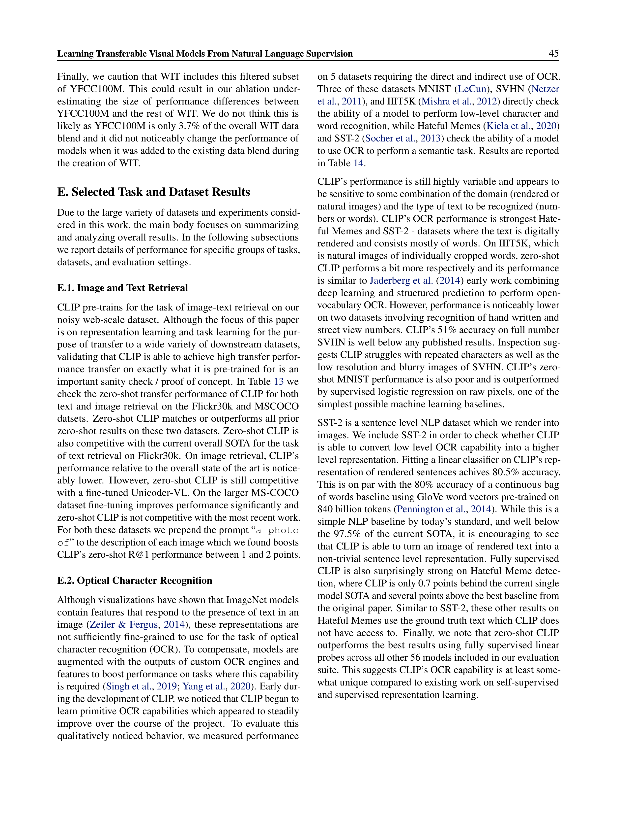
Learning Transferable Visual Models From Natural Language Supervision
45
Finally,
we
caution
that
WIT
includes
this
filtered
subset
of
YFCC100M.
This
could
result
in
our
ablation
under-
estimating
the
size
of
performance
differences
between
YFCC100M
and
the
rest
of
WIT.
We
do
not
think
this
is
likely as YFCC100M is only 3.7% of the overall WIT data
blend and it did not noticeably change the performance of
models when it was added to the existing data blend during
the creation of WIT.
E. Selected Task and Dataset Results
Due to the large variety of datasets and experiments consid-
ered in this work, the main body focuses on summarizing
and analyzing overall results.
In the following subsections
we report details of performance for specific groups of tasks,
datasets, and evaluation settings.
E.1. Image and Text Retrieval
CLIP pre-trains for the task of image-text retrieval on our
noisy web-scale dataset.
Although the focus of this paper
is on representation learning and task learning for the pur-
pose of transfer to a wide variety of downstream datasets,
validating that CLIP is able to achieve high transfer perfor-
mance
transfer
on
exactly
what
it
is
pre-trained
for
is
an
important sanity check / proof of concept.
In Table
13
we
check the zero-shot transfer performance of CLIP for both
text
and
image
retrieval
on
the
Flickr30k
and
MSCOCO
datsets.
Zero-shot CLIP matches or outperforms all prior
zero-shot results on these two datasets.
Zero-shot CLIP is
also competitive with the current overall SOTA for the task
of text retrieval on Flickr30k.
On image retrieval, CLIP’s
performance relative to the overall state of the art is notice-
ably
lower.
However,
zero-shot
CLIP
is
still
competitive
with a fine-tuned Unicoder-VL. On the larger MS-COCO
dataset fine-tuning improves performance significantly and
zero-shot CLIP is not competitive with the most recent work.
For both these datasets we prepend the prompt “
a
photo
of
” to the description of each image which we found boosts
CLIP’s zero-shot R@1 performance between 1 and 2 points.
E.2. Optical Character Recognition
Although visualizations have shown that ImageNet models
contain features that respond to the presence of text in an
image
(
Zeiler
&
Fergus
,
2014
),
these
representations
are
not
sufficiently
fine-grained
to
use
for
the
task
of
optical
character recognition (OCR). To compensate, models are
augmented
with
the
outputs
of
custom
OCR
engines
and
features to boost performance on tasks where this capability
is required (
Singh et al.
,
2019
;
Yang et al.
,
2020
).
Early dur-
ing the development of CLIP, we noticed that CLIP began to
learn primitive OCR capabilities which appeared to steadily
improve
over
the
course
of
the
project.
To
evaluate
this
qualitatively noticed behavior, we measured performance
on 5 datasets requiring the direct and indirect use of OCR.
Three
of
these
datasets
MNIST
(
LeCun
),
SVHN
(
Netzer
et al.
,
2011
), and IIIT5K (
Mishra et al.
,
2012
) directly check
the ability of a model to perform low-level character and
word recognition, while Hateful Memes (
Kiela et al.
,
2020
)
and SST-2 (
Socher et al.
,
2013
) check the ability of a model
to use OCR to perform a semantic task.
Results are reported
in Table
14
.
CLIP’s performance is still highly variable and appears to
be sensitive to some combination of the domain (rendered or
natural images) and the type of text to be recognized (num-
bers or words).
CLIP’s OCR performance is strongest Hate-
ful Memes and SST-2 - datasets where the text is digitally
rendered and consists mostly of words.
On IIIT5K, which
is natural images of individually cropped words, zero-shot
CLIP performs a bit more respectively and its performance
is similar to
Jaderberg et al.
(
2014
) early work combining
deep
learning
and
structured
prediction
to
perform
open-
vocabulary OCR. However, performance is noticeably lower
on two datasets involving recognition of hand written and
street view numbers.
CLIP’s 51% accuracy on full number
SVHN is well below any published results.
Inspection sug-
gests CLIP struggles with repeated characters as well as the
low resolution and blurry images of SVHN. CLIP’s zero-
shot MNIST performance is also poor and is outperformed
by supervised logistic regression on raw pixels, one of the
simplest possible machine learning baselines.
SST-2 is a sentence level NLP dataset which we render into
images.
We include SST-2 in order to check whether CLIP
is
able
to
convert
low
level
OCR
capability
into
a
higher
level representation.
Fitting a linear classifier on CLIP’s rep-
resentation of rendered sentences achives 80.5% accuracy.
This is on par with the 80% accuracy of a continuous bag
of words baseline using GloVe word vectors pre-trained on
840 billion tokens (
Pennington et al.
,
2014
).
While this is a
simple NLP baseline by today’s standard, and well below
the
97.5%
of
the
current
SOTA,
it
is
encouraging
to
see
that CLIP is able to turn an image of rendered text into a
non-trivial sentence level representation.
Fully supervised
CLIP
is
also
surprisingly
strong
on
Hateful
Meme
detec-
tion, where CLIP is only 0.7 points behind the current single
model SOTA and several points above the best baseline from
the original paper.
Similar to SST-2, these other results on
Hateful Memes use the ground truth text which CLIP does
not
have
access
to.
Finally,
we
note
that
zero-shot
CLIP
outperforms
the
best
results
using
fully
supervised
linear
probes across all other 56 models included in our evaluation
suite.
This suggests CLIP’s OCR capability is at least some-
what unique compared to existing work on self-supervised
and supervised representation learning.
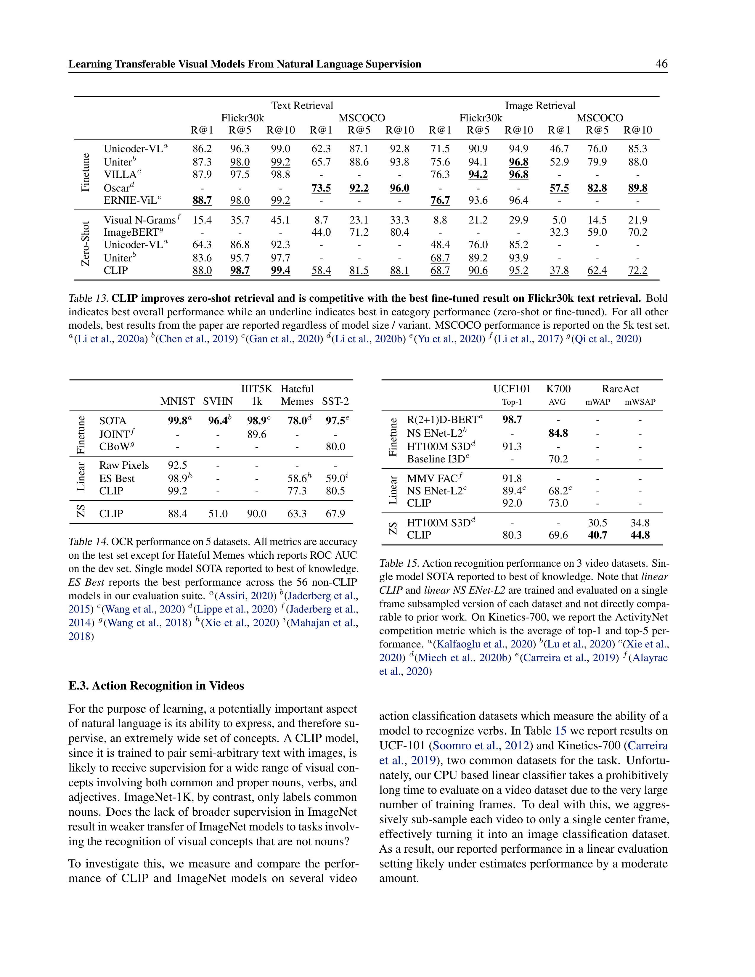
Learning Transferable Visual Models From Natural Language Supervision
46
Text Retrieval
Image Retrieval
Flickr30k
MSCOCO
Flickr30k
MSCOCO
R@1
R@5
R@10
R@1
R@5
R@10
R@1
R@5
R@10
R@1
R@5
R@10
Finetune
Unicoder-VL
a
86.2
96.3
99.0
62.3
87.1
92.8
71.5
90.9
94.9
46.7
76.0
85.3
Uniter
b
87.3
98.0
99.2
65.7
88.6
93.8
75.6
94.1
96.8
52.9
79.9
88.0
VILLA
c
87.9
97.5
98.8
-
-
-
76.3
94.2
96.8
-
-
-
Oscar
d
-
-
-
73.5
92.2
96.0
-
-
-
57.5
82.8
89.8
ERNIE-ViL
e
88.7
98.0
99.2
-
-
-
76.7
93.6
96.4
-
-
-
Zero-Shot
Visual N-Grams
f
15.4
35.7
45.1
8.7
23.1
33.3
8.8
21.2
29.9
5.0
14.5
21.9
ImageBERT
g
-
-
-
44.0
71.2
80.4
-
-
-
32.3
59.0
70.2
Unicoder-VL
a
64.3
86.8
92.3
-
-
-
48.4
76.0
85.2
-
-
-
Uniter
b
83.6
95.7
97.7
-
-
-
68.7
89.2
93.9
-
-
-
CLIP
88.0
98.7
99.4
58.4
81.5
88.1
68.7
90.6
95.2
37.8
62.4
72.2
Table 13.
CLIP improves zero-shot retrieval and is competitive with the best fine-tuned result on Flickr30k text retrieval.
Bold
indicates best overall performance while an underline indicates best in category performance (zero-shot or fine-tuned).
For all other
models, best results from the paper are reported regardless of model size / variant.
MSCOCO performance is reported on the 5k test set.
a
(
Li et al.
,
2020a
)
b
(
Chen et al.
,
2019
)
c
(
Gan et al.
,
2020
)
d
(
Li et al.
,
2020b
)
e
(
Yu et al.
,
2020
)
f
(
Li et al.
,
2017
)
g
(
Qi et al.
,
2020
)
IIIT5K
Hateful
MNIST
SVHN
1k
Memes
SST-2
Finetune
SOTA
99.8
a
96.4
b
98.9
c
78.0
d
97.5
e
JOINT
f
-
-
89.6
-
-
CBoW
g
-
-
-
-
80.0
Linear
Raw Pixels
92.5
-
-
-
-
ES Best
98.9
h
-
-
58.6
h
59.0
i
CLIP
99.2
-
-
77.3
80.5
ZS
CLIP
88.4
51.0
90.0
63.3
67.9
Table 14.
OCR performance on 5 datasets. All metrics are accuracy
on the test set except for Hateful Memes which reports ROC AUC
on the dev set.
Single model SOTA reported to best of knowledge.
ES
Best
reports
the
best
performance
across
the
56
non-CLIP
models in our evaluation suite.
a
(
Assiri
,
2020
)
b
(
Jaderberg et al.
,
2015
)
c
(
Wang et al.
,
2020
)
d
(
Lippe et al.
,
2020
)
f
(
Jaderberg et al.
,
2014
)
g
(
Wang et
al.
,
2018
)
h
(
Xie
et
al.
,
2020
)
i
(
Mahajan
et
al.
,
2018
)
E.3. Action Recognition in Videos
For the purpose of learning, a potentially important aspect
of natural language is its ability to express, and therefore su-
pervise, an extremely wide set of concepts.
A CLIP model,
since it is trained to pair semi-arbitrary text with images, is
likely to receive supervision for a wide range of visual con-
cepts involving both common and proper nouns, verbs, and
adjectives.
ImageNet-1K, by contrast, only labels common
nouns.
Does the lack of broader supervision in ImageNet
result in weaker transfer of ImageNet models to tasks involv-
ing the recognition of visual concepts that are not nouns?
To
investigate
this,
we
measure
and
compare
the
perfor-
mance
of
CLIP
and
ImageNet
models
on
several
video
UCF101
K700
RareAct
Top-1
AVG
mWAP
mWSAP
Finetune
R(2+1)D-BERT
a
98.7
-
-
-
NS ENet-L2
b
-
84.8
-
-
HT100M S3D
d
91.3
-
-
-
Baseline I3D
e
-
70.2
-
-
Linear
MMV FAC
f
91.8
-
-
-
NS ENet-L2
c
89.4
c
68.2
c
-
-
CLIP
92.0
73.0
-
-
ZS
HT100M S3D
d
-
-
30.5
34.8
CLIP
80.3
69.6
40.7
44.8
Table 15.
Action recognition performance on 3 video datasets.
Sin-
gle model SOTA reported to best of knowledge.
Note that
linear
CLIP
and
linear NS ENet-L2
are trained and evaluated on a single
frame subsampled version of each dataset and not directly compa-
rable to prior work.
On Kinetics-700, we report the ActivityNet
competition metric which is the average of top-1 and top-5 per-
formance.
a
(
Kalfaoglu et al.
,
2020
)
b
(
Lu et al.
,
2020
)
c
(
Xie et al.
,
2020
)
d
(
Miech
et
al.
,
2020b
)
e
(
Carreira
et
al.
,
2019
)
f
(
Alayrac
et al.
,
2020
)
action classification datasets which measure the ability of a
model to recognize verbs.
In Table
15
we report results on
UCF-101 (
Soomro et al.
,
2012
) and Kinetics-700 (
Carreira
et al.
,
2019
),
two common datasets for the task.
Unfortu-
nately, our CPU based linear classifier takes a prohibitively
long time to evaluate on a video dataset due to the very large
number
of
training
frames.
To
deal
with
this,
we
aggres-
sively sub-sample each video to only a single center frame,
effectively
turning
it
into
an
image
classification
dataset.
As a result, our reported performance in a linear evaluation
setting likely under estimates performance by a moderate
amount.
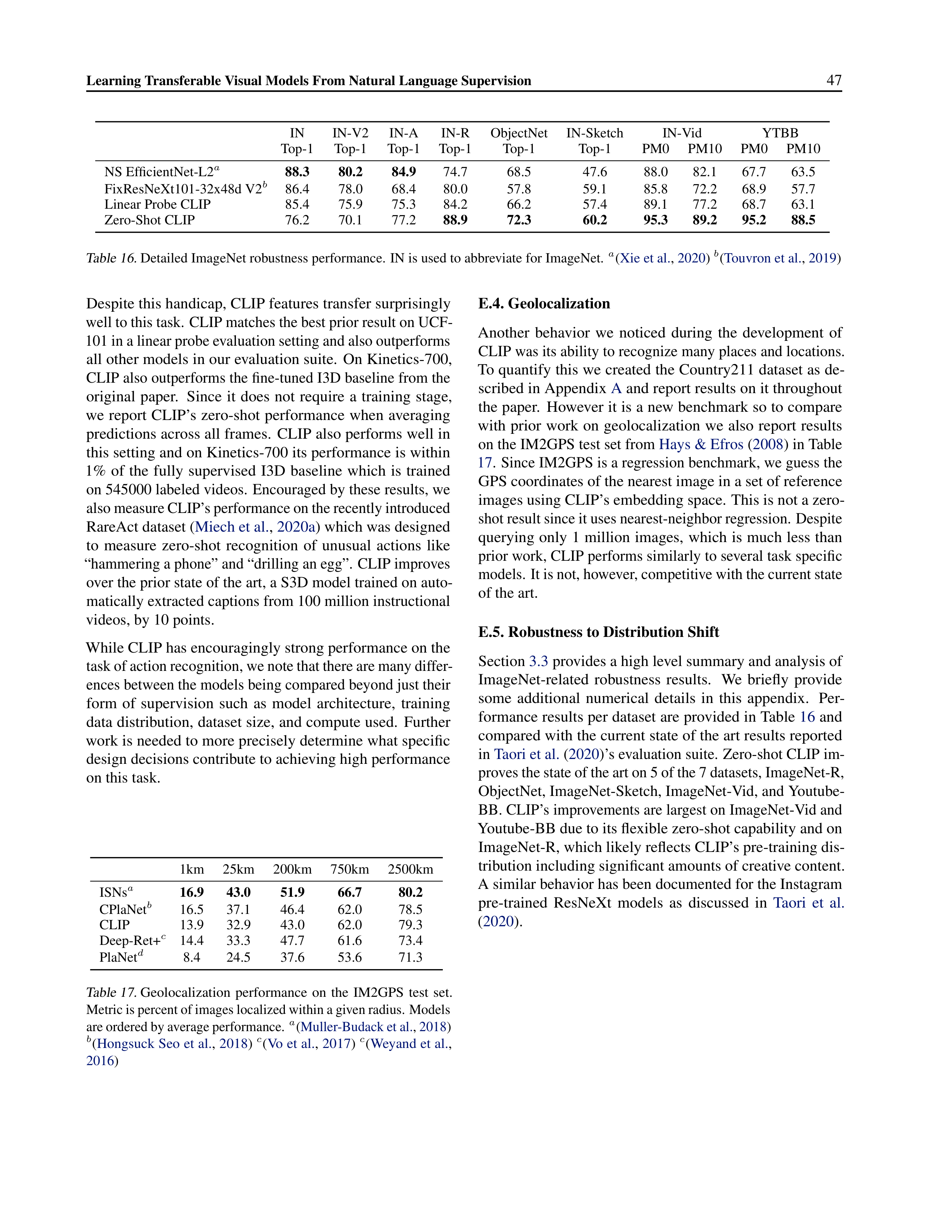
Learning Transferable Visual Models From Natural Language Supervision
47
IN
IN-V2
IN-A
IN-R
ObjectNet
IN-Sketch
IN-Vid
YTBB
Top-1
Top-1
Top-1
Top-1
Top-1
Top-1
PM0
PM10
PM0
PM10
NS EfficientNet-L2
a
88.3
80.2
84.9
74.7
68.5
47.6
88.0
82.1
67.7
63.5
FixResNeXt101-32x48d V2
b
86.4
78.0
68.4
80.0
57.8
59.1
85.8
72.2
68.9
57.7
Linear Probe CLIP
85.4
75.9
75.3
84.2
66.2
57.4
89.1
77.2
68.7
63.1
Zero-Shot CLIP
76.2
70.1
77.2
88.9
72.3
60.2
95.3
89.2
95.2
88.5
Table 16.
Detailed ImageNet robustness performance.
IN is used to abbreviate for ImageNet.
a
(
Xie et al.
,
2020
)
b
(
Touvron et al.
,
2019
)
Despite this handicap, CLIP features transfer surprisingly
well to this task.
CLIP matches the best prior result on UCF-
101 in a linear probe evaluation setting and also outperforms
all other models in our evaluation suite.
On Kinetics-700,
CLIP also outperforms the fine-tuned I3D baseline from the
original
paper.
Since
it
does
not
require
a
training
stage,
we
report
CLIP’s
zero-shot
performance
when
averaging
predictions across all frames.
CLIP also performs well in
this setting and on Kinetics-700 its performance is within
1%
of
the
fully
supervised
I3D
baseline
which
is
trained
on 545000 labeled videos.
Encouraged by these results, we
also measure CLIP’s performance on the recently introduced
RareAct dataset (
Miech et al.
,
2020a
) which was designed
to
measure
zero-shot
recognition
of
unusual
actions
like
“hammering a phone” and “drilling an egg”.
CLIP improves
over the prior state of the art, a S3D model trained on auto-
matically extracted captions from 100 million instructional
videos, by 10 points.
While CLIP has encouragingly strong performance on the
task of action recognition, we note that there are many differ-
ences between the models being compared beyond just their
form
of
supervision
such
as
model
architecture,
training
data distribution, dataset size, and compute used.
Further
work is needed to more precisely determine what specific
design decisions contribute to achieving high performance
on this task.
1km
25km
200km
750km
2500km
ISNs
a
16.9
43.0
51.9
66.7
80.2
CPlaNet
b
16.5
37.1
46.4
62.0
78.5
CLIP
13.9
32.9
43.0
62.0
79.3
Deep-Ret+
c
14.4
33.3
47.7
61.6
73.4
PlaNet
d
8.4
24.5
37.6
53.6
71.3
Table 17.
Geolocalization
performance
on
the
IM2GPS
test
set.
Metric is percent of images localized within a given radius. Models
are ordered by average performance.
a
(
Muller-Budack et al.
,
2018
)
b
(
Hongsuck Seo et al.
,
2018
)
c
(
Vo et al.
,
2017
)
c
(
Weyand et al.
,
2016
)
E.4. Geolocalization
Another
behavior
we
noticed
during
the
development
of
CLIP was its ability to recognize many places and locations.
To quantify this we created the Country211 dataset as de-
scribed in Appendix
A
and report results on it throughout
the paper.
However it is a new benchmark so to compare
with
prior
work
on
geolocalization
we
also
report
results
on the IM2GPS test set from
Hays & Efros
(
2008
) in Table
17
.
Since IM2GPS is a regression benchmark, we guess the
GPS coordinates of the nearest image in a set of reference
images using CLIP’s embedding space.
This is not a zero-
shot result since it uses nearest-neighbor regression.
Despite
querying only 1 million images,
which is much less than
prior work, CLIP performs similarly to several task specific
models.
It is not, however, competitive with the current state
of the art.
E.5. Robustness to Distribution Shift
Section
3.3
provides a high level summary and analysis of
ImageNet-related
robustness
results.
We
briefly
provide
some
additional
numerical
details
in
this
appendix.
Per-
formance results per dataset are provided in Table
16
and
compared with the current state of the art results reported
in
Taori et al.
(
2020
)’s evaluation suite.
Zero-shot CLIP im-
proves the state of the art on 5 of the 7 datasets, ImageNet-R,
ObjectNet, ImageNet-Sketch, ImageNet-Vid, and Youtube-
BB. CLIP’s improvements are largest on ImageNet-Vid and
Youtube-BB due to its flexible zero-shot capability and on
ImageNet-R, which likely reflects CLIP’s pre-training dis-
tribution including significant amounts of creative content.
A similar behavior has been documented for the Instagram
pre-trained
ResNeXt
models
as
discussed
in
Taori
et
al.
(
2020
).
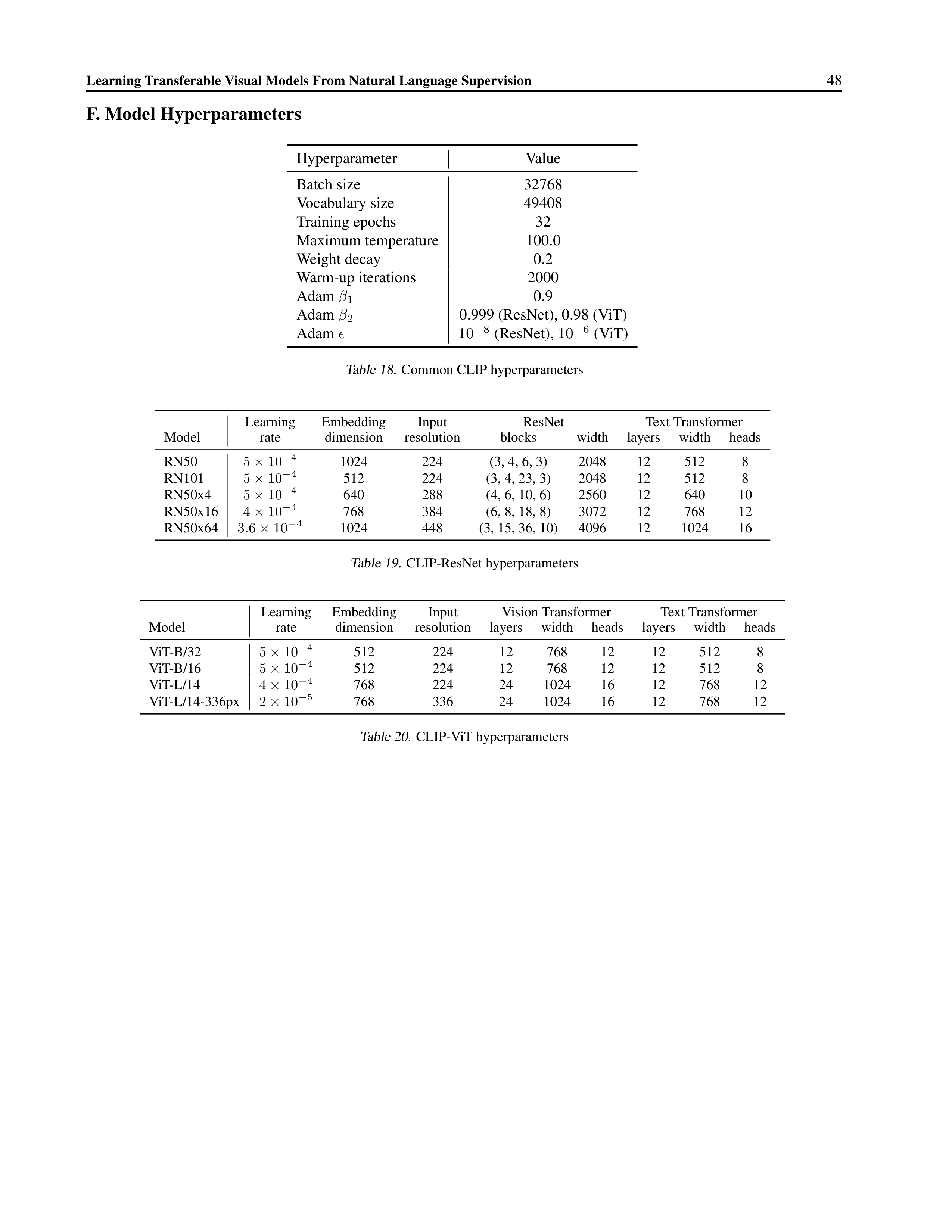
Learning Transferable Visual Models From Natural Language Supervision
48
F. Model Hyperparameters
Hyperparameter
Value
Batch size
32768
Vocabulary size
49408
Training epochs
32
Maximum temperature
100.0
Weight decay
0.2
Warm-up iterations
2000
Adam
β
1
0.9
Adam
β
2
0.999 (ResNet), 0.98 (ViT)
Adam
ϵ
10
−
8
(ResNet),
10
−
6
(ViT)
Table 18.
Common CLIP hyperparameters
Learning
Embedding
Input
ResNet
Text Transformer
Model
rate
dimension
resolution
blocks
width
layers
width
heads
RN50
5
×
10
−
4
1024
224
(3, 4, 6, 3)
2048
12
512
8
RN101
5
×
10
−
4
512
224
(3, 4, 23, 3)
2048
12
512
8
RN50x4
5
×
10
−
4
640
288
(4, 6, 10, 6)
2560
12
640
10
RN50x16
4
×
10
−
4
768
384
(6, 8, 18, 8)
3072
12
768
12
RN50x64
3
.
6
×
10
−
4
1024
448
(3, 15, 36, 10)
4096
12
1024
16
Table 19.
CLIP-ResNet hyperparameters
Learning
Embedding
Input
Vision Transformer
Text Transformer
Model
rate
dimension
resolution
layers
width
heads
layers
width
heads
ViT-B/32
5
×
10
−
4
512
224
12
768
12
12
512
8
ViT-B/16
5
×
10
−
4
512
224
12
768
12
12
512
8
ViT-L/14
4
×
10
−
4
768
224
24
1024
16
12
768
12
ViT-L/14-336px
2
×
10
−
5
768
336
24
1024
16
12
768
12
Table 20.
CLIP-ViT hyperparameters