Deep Residual Learning for Image Recognition
Kaiming He
Xiangyu Zhang
Shaoqing Ren
Jian Sun
Microsoft Research
{
kahe, v-xiangz, v-shren, jiansun
}
@microsoft.com
Abstract
Deeper
neural
networks
are
more
difficult
to
train.
We
present a residual learning framework to ease the training
of
networks
that
are
substantially
deeper
than
those
used
previously.
We
explicitly
reformulate
the
layers
as
learn-
ing residual functions with reference to the layer inputs, in-
stead of learning unreferenced functions.
We provide com-
prehensive
empirical
evidence
showing
that
these
residual
networks are easier to optimize, and can gain accuracy from
considerably increased depth.
On the ImageNet dataset we
evaluate residual nets with a depth of up to 152 layers—8
×
deeper than VGG nets [41] but still having lower complex-
ity. An ensemble of these residual nets achieves 3.57% error
on the ImageNet
test
set. This result won the 1st place on the
ILSVRC 2015 classification
task.
We
also
present
analysis
on CIFAR-10 with 100 and 1000 layers.
The
depth
of
representations
is
of
central
importance
for
many
visual
recognition
tasks.
Solely
due
to
our
ex-
tremely deep representations, we obtain a 28% relative im-
provement
on
the
COCO
object
detection
dataset.
Deep
residual nets are foundations of our submissions to ILSVRC
&
COCO
2015
competitions
1
,
where
we
also
won
the
1st
places on the tasks of ImageNet detection, ImageNet local-
ization, COCO detection, and COCO segmentation.
1. Introduction
Deep
convolutional
neural
networks
[22,
21]
have
led
to
a
series
of
breakthroughs
for
image
classification
[21,
50,
40].
Deep
networks
naturally
integrate
low/mid/high-
level
features
[50]
and
classifiers
in
an
end-to-end
multi-
layer
fashion,
and
the
“levels”
of
features
can
be
enriched
by
the
number
of
stacked
layers
(depth).
Recent
evidence
[41, 44] reveals that network depth is of crucial importance,
and
the
leading
results
[41,
44,
13,
16]
on
the
challenging
ImageNet dataset [36] all exploit “very deep” [41] models,
with a depth of sixteen [41] to thirty [16].
Many other non-
trivial
visual
recognition
tasks
[8,
12,
7,
32,
27]
have
also
1
http://image-net.org/challenges/LSVRC/2015/
and
http://mscoco.org/dataset/#detections-challenge2015
.
0
1
2
3
4
5
6
0
10
20
iter. (1e4)
training error (%)
0
1
2
3
4
5
6
0
10
20
iter. (1e4)
test error (%)
56-layer
20-layer
56-layer
20-layer
Figure
1.
Training
error
(left)
and
test
error
(right)
on
CIFAR-10
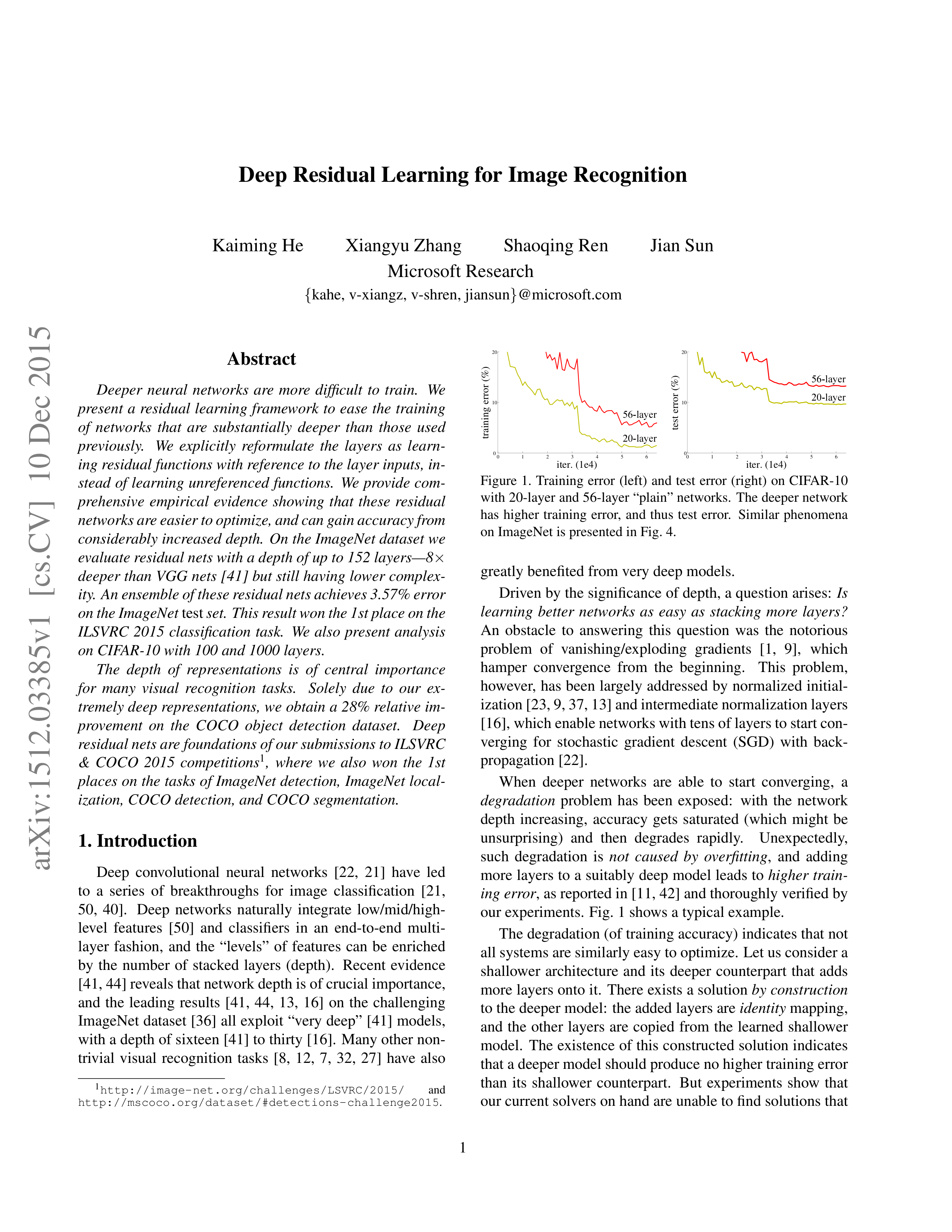
with 20-layer and 56-layer “plain” networks.
The deeper network
has
higher
training
error,
and
thus
test
error.
Similar
phenomena
on ImageNet is presented in Fig. 4.
greatly benefited from very deep models.
Driven by the significance of depth, a question arises:
Is
learning
better
networks
as
easy
as
stacking
more
layers?
An
obstacle
to
answering
this
question
was
the
notorious
problem
of
vanishing/exploding
gradients
[1,
9],
which
hamper
convergence
from
the
beginning.
This
problem,
however, has been largely addressed by normalized initial-
ization [23, 9, 37, 13] and intermediate normalization layers
[16], which enable networks with tens of layers to start con-
verging
for
stochastic
gradient
descent
(SGD)
with
back-
propagation [22].
When
deeper
networks
are
able
to
start
converging,
a
degradation
problem
has
been
exposed:
with
the
network
depth
increasing,
accuracy
gets
saturated
(which
might
be
unsurprising)
and
then
degrades
rapidly.
Unexpectedly,
such
degradation
is
not
caused
by
overfitting
,
and
adding
more layers to a suitably deep model leads to
higher train-
ing error
, as reported in [11, 42] and thoroughly verified by
our experiments.
Fig. 1 shows a typical example.
The degradation (of training accuracy) indicates that not
all systems are similarly easy to optimize.
Let us consider a
shallower
architecture
and
its
deeper
counterpart
that
adds
more layers onto it.
There exists a solution
by construction
to the deeper model:
the added layers are
identity
mapping,
and
the
other
layers
are
copied
from
the
learned
shallower
model.
The existence of this constructed solution indicates
that a deeper model should produce no higher training error
than
its
shallower
counterpart.
But
experiments
show
that
our current solvers on hand are unable to find solutions that
1
arXiv:1512.03385v1 [cs.CV] 10 Dec 2015
identity
weight layer
weight layer
relu
relu
F
(
x
)
+
x
x
F
(
x
)
x
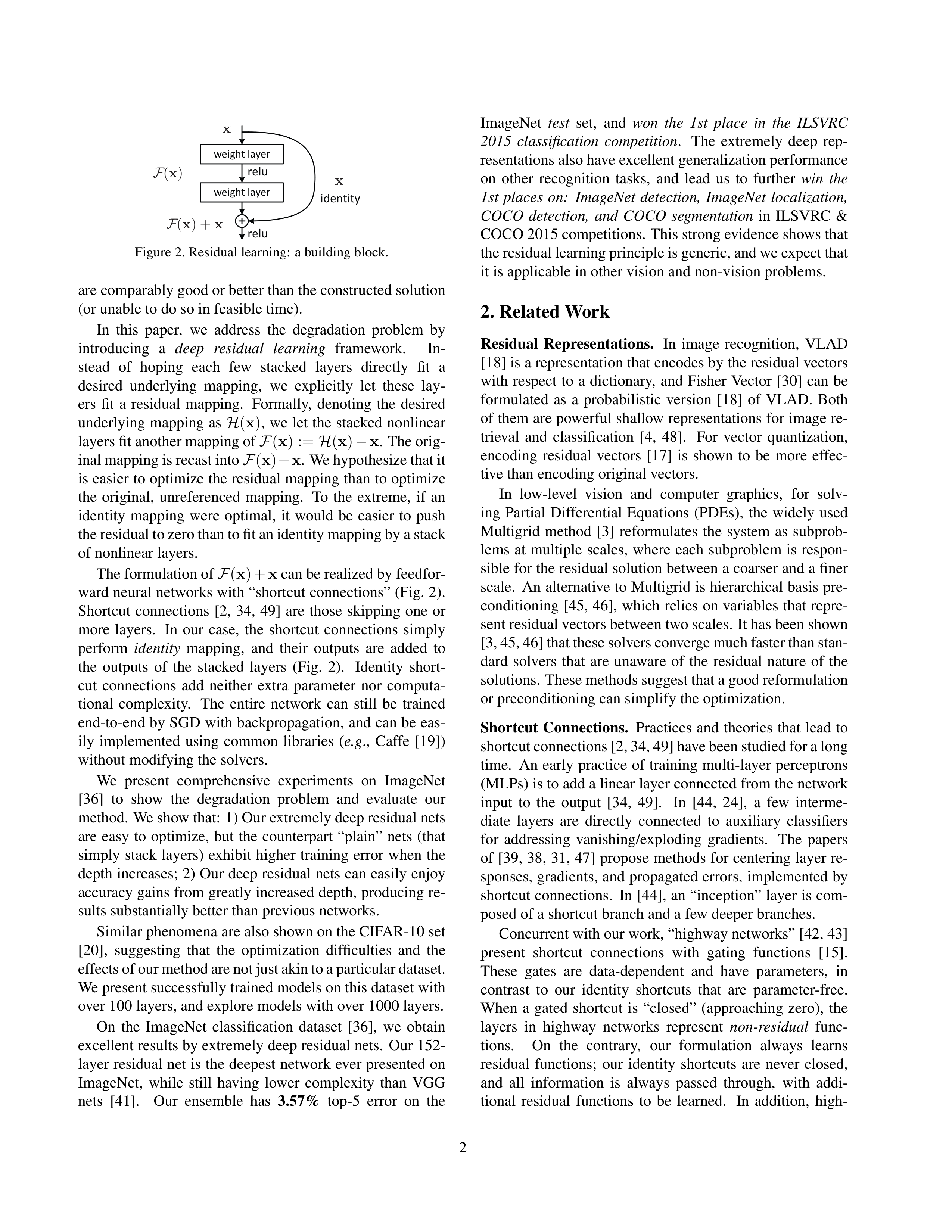
Figure 2. Residual learning:
a building block.
are comparably good or better than the constructed solution
(or unable to do so in feasible time).
In
this
paper,
we
address
the
degradation
problem
by
introducing
a
deep
residual
learning
framework.
In-
stead
of
hoping
each
few
stacked
layers
directly
fit
a
desired
underlying
mapping,
we
explicitly
let
these
lay-
ers
fit
a
residual
mapping.
Formally,
denoting
the
desired
underlying mapping as
H
(
x
)
,
we let the
stacked
nonlinear
layers fit another mapping of
F
(
x
) :=
H
(
x
)
−
x
.
The orig-
inal mapping is recast into
F
(
x
)+
x
. We hypothesize that it
is easier to optimize the residual mapping than to optimize
the
original,
unreferenced
mapping.
To
the
extreme,
if
an
identity
mapping
were
optimal,
it
would
be
easier
to
push
the residual to zero than to fit an identity mapping by a stack
of nonlinear layers.
The formulation of
F
(
x
)+
x
can be realized by feedfor-
ward neural networks with “shortcut connections” (Fig. 2).
Shortcut
connections
[2,
34,
49]
are
those
skipping
one
or
more
layers.
In
our
case,
the
shortcut
connections
simply
perform
identity
mapping,
and
their
outputs
are
added
to
the
outputs
of
the
stacked
layers
(Fig.
2).
Identity
short-
cut
connections
add
neither
extra
parameter
nor
computa-
tional
complexity.
The
entire
network
can
still
be
trained
end-to-end by SGD with backpropagation, and can be eas-
ily
implemented
using
common
libraries
(
e.g
.,
Caffe
[19])
without modifying the solvers.
We
present
comprehensive
experiments
on
ImageNet
[36]
to
show
the
degradation
problem
and
evaluate
our
method.
We show that:
1) Our extremely deep residual nets
are
easy
to
optimize,
but
the
counterpart
“plain”
nets
(that
simply
stack
layers)
exhibit
higher
training
error
when
the
depth increases; 2) Our deep residual nets can easily enjoy
accuracy gains from greatly increased depth, producing re-
sults substantially better than previous networks.
Similar phenomena are also shown on the CIFAR-10 set
[20],
suggesting
that
the
optimization
difficulties
and
the
effects of our method are not just akin to a particular dataset.
We present successfully trained models on this dataset with
over 100 layers, and explore models with over 1000 layers.
On
the
ImageNet
classification
dataset
[36],
we
obtain
excellent results by extremely deep residual nets.
Our 152-
layer residual net is the deepest network ever presented on
ImageNet,
while
still
having
lower
complexity
than
VGG
nets
[41].
Our
ensemble
has
3.57%
top-5
error
on
the
ImageNet
test
set,
and
won
the
1st
place
in
the
ILSVRC
2015
classification
competition
.
The
extremely
deep
rep-
resentations also have excellent generalization performance
on
other
recognition
tasks,
and
lead
us
to
further
win
the
1st
places
on:
ImageNet
detection,
ImageNet
localization,
COCO
detection,
and
COCO
segmentation
in
ILSVRC
&
COCO 2015 competitions.
This strong evidence shows that
the residual learning principle is generic, and we expect that
it is applicable in other vision and non-vision problems.
2. Related Work
Residual
Representations.
In
image
recognition,
VLAD
[18] is a representation that encodes by the residual vectors
with
respect
to
a
dictionary,
and
Fisher
Vector
[30]
can
be
formulated
as
a
probabilistic
version
[18]
of
VLAD.
Both
of them are powerful shallow representations for image re-
trieval
and
classification
[4,
48].
For
vector
quantization,
encoding
residual
vectors
[17]
is
shown
to
be
more
effec-
tive than encoding original vectors.
In
low-level
vision
and
computer
graphics,
for
solv-
ing
Partial
Differential
Equations
(PDEs),
the
widely
used
Multigrid
method
[3]
reformulates
the
system
as
subprob-
lems
at
multiple
scales,
where
each
subproblem
is
respon-
sible for the residual solution between a coarser and a finer
scale.
An alternative to Multigrid is hierarchical basis pre-
conditioning [45, 46],
which relies on variables that repre-
sent residual vectors between two scales.
It has been shown
[3, 45, 46] that these solvers converge much faster than stan-
dard
solvers
that
are
unaware
of
the
residual
nature
of
the
solutions.
These methods suggest that a good reformulation
or preconditioning can simplify the optimization.
Shortcut
Connections.
Practices
and
theories
that
lead
to
shortcut connections [2, 34, 49] have been studied for a long
time.
An early practice of training multi-layer perceptrons
(MLPs) is to add a linear layer connected from the network
input
to
the
output
[34,
49].
In
[44,
24],
a
few
interme-
diate
layers
are
directly
connected
to
auxiliary
classifiers
for
addressing
vanishing/exploding
gradients.
The
papers
of [39, 38, 31, 47] propose methods for centering layer re-
sponses, gradients, and propagated errors, implemented by
shortcut connections.
In [44], an “inception” layer is com-
posed of a shortcut branch and a few deeper branches.
Concurrent with our work, “highway networks” [42, 43]
present
shortcut
connections
with
gating
functions
[15].
These
gates
are
data-dependent
and
have
parameters,
in
contrast
to
our
identity
shortcuts
that
are
parameter-free.
When
a
gated
shortcut
is
“closed”
(approaching
zero),
the
layers
in
highway
networks
represent
non-residual
func-
tions.
On
the
contrary,
our
formulation
always
learns
residual
functions;
our
identity
shortcuts
are
never
closed,
and
all
information
is
always
passed
through,
with
addi-
tional
residual
functions
to
be
learned.
In
addition,
high-
2
way
networks
have
not
demonstrated
accuracy
gains
with
extremely increased depth (
e.g
., over 100 layers).
3. Deep Residual Learning
3.1. Residual Learning
Let
us
consider
H
(
x
)
as
an
underlying
mapping
to
be
fit
by
a
few
stacked
layers
(not
necessarily
the
entire
net),
with
x
denoting the inputs to the first of these layers.
If one
hypothesizes
that
multiple
nonlinear
layers
can
asymptoti-
cally approximate complicated functions
2
, then it is equiv-
alent
to
hypothesize
that
they
can
asymptotically
approxi-
mate
the
residual
functions,
i.e
.,
H
(
x
)
−
x
(assuming
that
the
input
and
output
are
of
the
same
dimensions).
So
rather than expect stacked layers to approximate
H
(
x
)
, we
explicitly
let
these
layers
approximate
a
residual
function
F
(
x
)
:=
H
(
x
)
−
x
.
The
original
function
thus
becomes
F
(
x
)+
x
. Although both forms should be able to asymptot-
ically approximate the desired functions (as hypothesized),
the ease of learning might be different.
This
reformulation
is
motivated
by
the
counterintuitive
phenomena about the degradation problem (Fig. 1, left).
As
we
discussed
in
the
introduction,
if
the
added
layers
can
be constructed as identity mappings, a deeper model should
have
training
error
no
greater
than
its
shallower
counter-
part.
The
degradation
problem
suggests
that
the
solvers
might have difficulties in approximating identity mappings
by multiple nonlinear layers.
With the residual learning re-
formulation,
if
identity
mappings
are
optimal,
the
solvers
may simply drive the weights of the multiple nonlinear lay-
ers toward zero to approach identity mappings.
In real cases, it is unlikely that identity mappings are op-
timal,
but
our
reformulation
may
help
to
precondition
the
problem.
If
the
optimal
function
is
closer
to
an
identity
mapping than to a zero mapping, it should be easier for the
solver to find the perturbations with reference to an identity
mapping, than to learn the function as a new one.
We show
by experiments (Fig. 7) that the learned residual functions in
general have small responses, suggesting that identity map-
pings provide reasonable preconditioning.
3.2. Identity Mapping by Shortcuts
We
adopt
residual
learning
to
every
few
stacked
layers.
A building block is shown in Fig. 2.
Formally, in this paper
we consider a building block defined as:
y
=
F
(
x
,
{
W
i
}
) +
x
.
(1)
Here
x
and
y
are
the
input
and
output
vectors
of
the
lay-
ers
considered.
The
function
F
(
x
,
{
W
i
}
)
represents
the
residual
mapping
to
be
learned.
For
the
example
in
Fig.
2
that
has
two
layers,
F
=
W
2
σ
(
W
1
x
)
in
which
σ
denotes
2
This hypothesis, however, is still an open question.
See [28].
ReLU
[29]
and
the
biases
are
omitted
for
simplifying
no-
tations.
The
operation
F
+
x
is
performed
by
a
shortcut
connection
and
element-wise
addition.
We
adopt
the
sec-
ond nonlinearity after the addition (
i.e
.,
σ
(
y
)
, see Fig. 2).
The shortcut connections in Eqn.(1) introduce neither ex-
tra parameter nor computation complexity.
This is not only
attractive in practice but also important in our comparisons
between
plain
and
residual
networks.
We
can
fairly
com-
pare
plain/residual
networks
that
simultaneously
have
the
same
number
of
parameters,
depth,
width,
and
computa-
tional cost (except for the negligible element-wise addition).
The
dimensions
of
x
and
F
must
be
equal
in
Eqn.(1).
If this is not the case (
e.g
., when changing the input/output
channels),
we
can
perform
a
linear
projection
W
s
by
the
shortcut connections to match the dimensions:
y
=
F
(
x
,
{
W
i
}
) +
W
s
x
.
(2)
We can also use a square matrix
W
s
in Eqn.(1).
But we will
show by experiments that the identity mapping is sufficient
for addressing the degradation problem and is economical,
and thus
W
s
is only used when matching dimensions.
The
form
of
the
residual
function
F
is
flexible.
Exper-
iments
in
this
paper
involve
a
function
F
that
has
two
or
three layers (Fig. 5), while more layers are possible.
But if
F
has only a single layer, Eqn.(1) is similar to a linear layer:
y
=
W
1
x
+
x
, for which we have not observed advantages.
We also note that although the above notations are about
fully-connected layers for simplicity, they are applicable to
convolutional
layers.
The
function
F
(
x
,
{
W
i
}
)
can
repre-
sent multiple convolutional layers.
The element-wise addi-
tion is performed on two feature maps, channel by channel.
3.3. Network Architectures
We have tested various plain/residual nets, and have ob-
served consistent phenomena.
To provide instances for dis-
cussion, we describe two models for ImageNet as follows.
Plain
Network.
Our
plain
baselines
(Fig.
3,
middle)
are
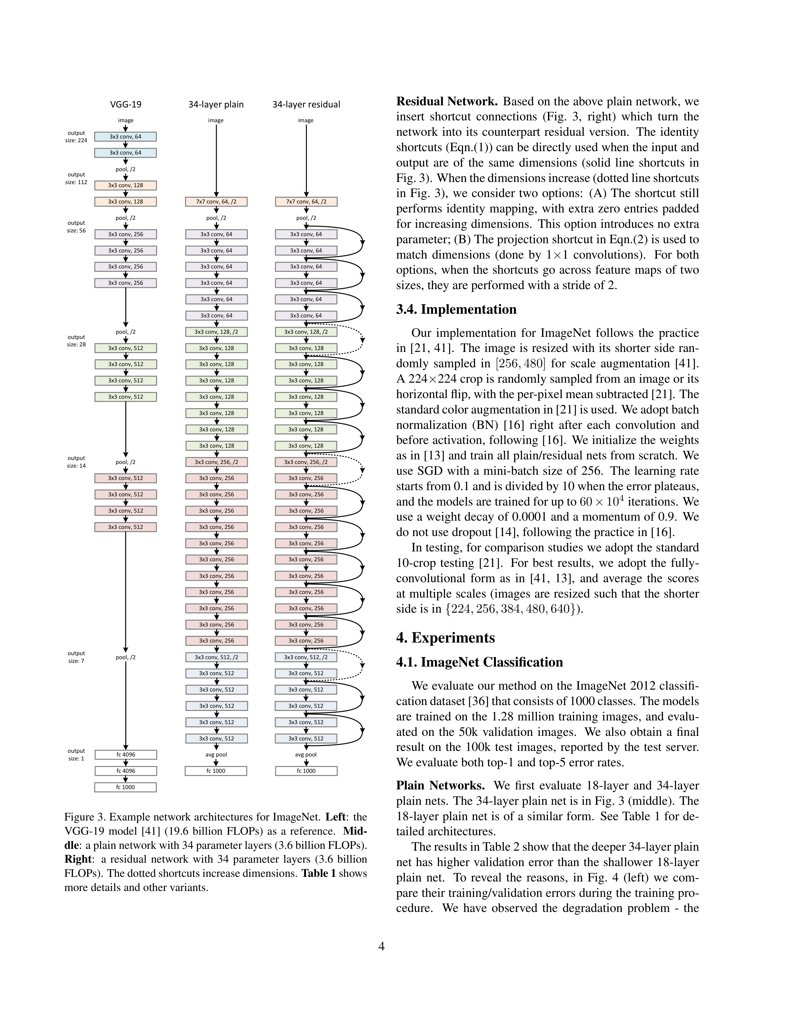
mainly inspired by the philosophy of VGG nets [41] (Fig. 3,
left).
The convolutional layers mostly have 3
×
3 filters and
follow
two
simple
design
rules:
(i)
for
the
same
output
feature
map
size,
the
layers
have
the
same
number
of
fil-
ters;
and
(ii)
if
the
feature
map
size
is
halved,
the
num-
ber
of
filters
is
doubled
so
as
to
preserve
the
time
com-
plexity
per
layer.
We
perform
downsampling
directly
by
convolutional
layers
that
have
a
stride
of
2.
The
network
ends
with
a
global
average
pooling
layer
and
a
1000-way
fully-connected
layer
with
softmax.
The
total
number
of
weighted layers is 34 in Fig. 3 (middle).
It
is
worth
noticing
that
our
model
has
fewer
filters
and
lower
complexity than VGG nets [41] (Fig. 3, left).
Our 34-
layer baseline has 3.6 billion FLOPs (multiply-adds), which
is only 18% of VGG-19 (19.6 billion FLOPs).
3
7x7 conv, 64, /2
pool, /2
3x3 conv, 64
3x3 conv, 64
3x3 conv, 64
3x3 conv, 64
3x3 conv, 64
3x3 conv, 64
3x3 conv, 128, /2
3x3 conv, 128
3x3 conv, 128
3x3 conv, 128
3x3 conv, 128
3x3 conv, 128
3x3 conv, 128
3x3 conv, 128
3x3 conv, 256, /2
3x3 conv, 256
3x3 conv, 256
3x3 conv, 256
3x3 conv, 256
3x3 conv, 256
3x3 conv, 256
3x3 conv, 256
3x3 conv, 256
3x3 conv, 256
3x3 conv, 256
3x3 conv, 256
3x3 conv, 512, /2
3x3 conv, 512
3x3 conv, 512
3x3 conv, 512
3x3 conv, 512
3x3 conv, 512
avg pool
fc 1000
image
3x3 conv, 512
3x3 conv, 64
3x3 conv, 64
pool, /2
3x3 conv, 128
3x3 conv, 128
pool, /2
3x3 conv, 256
3x3 conv, 256
3x3 conv, 256
3x3 conv, 256
pool, /2
3x3 conv, 512
3x3 conv, 512
3x3 conv, 512
pool, /2
3x3 conv, 512
3x3 conv, 512
3x3 conv, 512
3x3 conv, 512
pool, /2
fc 4096
fc 4096
fc 1000
image
output
size: 112
output
size: 224
output
size: 56
output
size: 28
output
size: 14
output
size: 7
output
size: 1
VGG-19
34-layer plain
7x7 conv, 64, /2
pool, /2
3x3 conv, 64
3x3 conv, 64
3x3 conv, 64
3x3 conv, 64
3x3 conv, 64
3x3 conv, 64
3x3 conv, 128, /2
3x3 conv, 128
3x3 conv, 128
3x3 conv, 128
3x3 conv, 128
3x3 conv, 128
3x3 conv, 128
3x3 conv, 128
3x3 conv, 256, /2
3x3 conv, 256
3x3 conv, 256
3x3 conv, 256
3x3 conv, 256
3x3 conv, 256
3x3 conv, 256
3x3 conv, 256
3x3 conv, 256
3x3 conv, 256
3x3 conv, 256
3x3 conv, 256
3x3 conv, 512, /2
3x3 conv, 512
3x3 conv, 512
3x3 conv, 512
3x3 conv, 512
3x3 conv, 512
avg pool
fc 1000
image
34-layer residual
Figure 3. Example network architectures for ImageNet.
Left
:
the
VGG-19
model
[41]
(19.6
billion
FLOPs)
as
a
reference.
Mid-
dle
: a plain network with 34 parameter layers (3.6 billion FLOPs).
Right
:
a
residual
network
with
34
parameter
layers
(3.6
billion
FLOPs). The dotted shortcuts increase dimensions.
Table 1
shows
more details and other variants.
Residual Network.
Based on the above plain network, we
insert
shortcut
connections
(Fig.
3,
right)
which
turn
the
network
into
its
counterpart
residual
version.
The
identity
shortcuts (Eqn.(1)) can be directly used when the input and
output
are
of
the
same
dimensions
(solid
line
shortcuts
in
Fig. 3). When the dimensions increase (dotted line shortcuts
in
Fig.
3),
we
consider
two
options:
(A)
The
shortcut
still
performs
identity
mapping,
with
extra
zero
entries
padded
for increasing dimensions.
This option introduces no extra
parameter; (B) The projection shortcut in Eqn.(2) is used to
match
dimensions
(done
by
1
×
1
convolutions).
For
both
options,
when
the
shortcuts
go
across
feature
maps
of
two
sizes, they are performed with a stride of 2.
3.4. Implementation
Our
implementation
for
ImageNet
follows
the
practice
in
[21,
41].
The
image
is
resized
with
its
shorter
side
ran-
domly
sampled
in
[256
,
480]
for
scale
augmentation
[41].
A 224
×
224 crop is randomly sampled from an image or its
horizontal flip, with the per-pixel mean subtracted [21]. The
standard color augmentation in [21] is used. We adopt batch
normalization
(BN)
[16]
right
after
each
convolution
and
before activation, following [16].
We initialize the weights
as in [13] and train all plain/residual nets from scratch.
We
use
SGD
with
a
mini-batch
size
of
256.
The
learning
rate
starts from 0.1 and is divided by 10 when the error plateaus,
and the models are trained for up to
60
×
10
4
iterations.
We
use a weight decay of 0.0001 and a momentum of 0.9.
We
do not use dropout [14], following the practice in [16].
In testing, for comparison studies we adopt the standard
10-crop
testing
[21].
For
best
results,
we
adopt
the
fully-
convolutional
form
as
in
[41,
13],
and
average
the
scores
at
multiple
scales
(images
are
resized
such
that
the
shorter
side is in
{
224
,
256
,
384
,
480
,
640
}
).
4. Experiments
4.1. ImageNet Classification
We evaluate our method on the ImageNet 2012 classifi-
cation dataset [36] that consists of 1000 classes. The models
are
trained
on
the
1.28
million
training
images,
and
evalu-
ated
on
the
50k
validation
images.
We
also
obtain
a
final
result
on
the
100k
test
images,
reported
by
the
test
server.
We evaluate both top-1 and top-5 error rates.
Plain
Networks.
We
first
evaluate
18-layer
and
34-layer
plain nets.
The 34-layer plain net is in Fig. 3 (middle).
The
18-layer plain net is of a similar form.
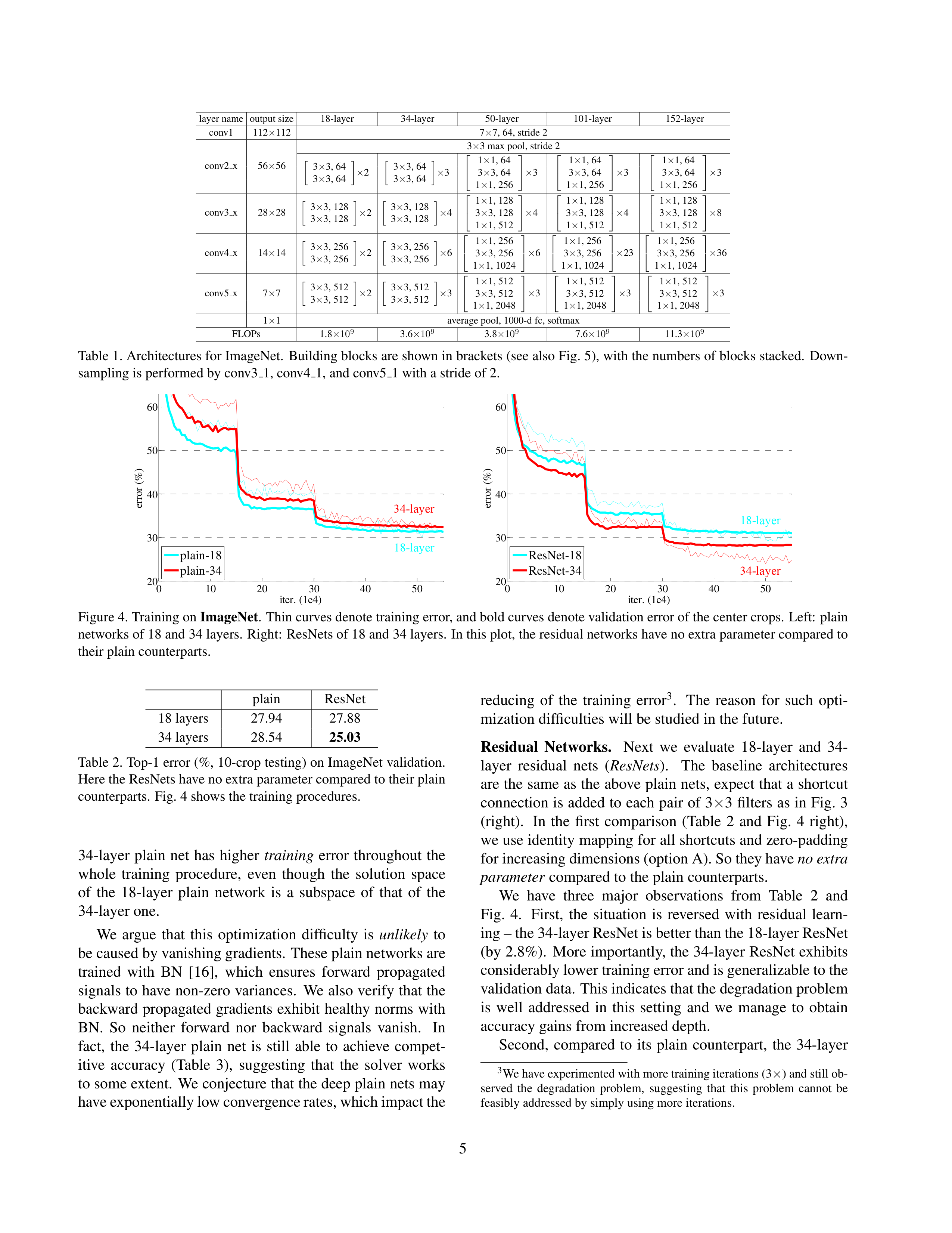
See Table 1 for de-
tailed architectures.
The results in Table 2 show that the deeper 34-layer plain
net
has
higher
validation
error
than
the
shallower
18-layer
plain
net.
To
reveal
the
reasons,
in
Fig.
4
(left)
we
com-
pare their training/validation errors during the training pro-
cedure.
We
have
observed
the
degradation
problem
-
the
4
layer name
output size
18-layer
34-layer
50-layer
101-layer
152-layer
conv1
112
×
112
7
×
7, 64, stride 2
conv2
x
56
×
56
3
×
3 max pool, stride 2
3
×
3, 64
3
×
3, 64
×
2
3
×
3, 64
3
×
3, 64
×
3
1
×
1, 64
3
×
3, 64
1
×
1, 256
×
3
1
×
1, 64
3
×
3, 64
1
×
1, 256
×
3
1
×
1, 64
3
×
3, 64
1
×
1, 256
×
3
conv3
x
28
×
28
3
×
3, 128
3
×
3, 128
×
2
3
×
3, 128
3
×
3, 128
×
4
1
×
1, 128
3
×
3, 128
1
×
1, 512
×
4
1
×
1, 128
3
×
3, 128
1
×
1, 512
×
4
1
×
1, 128
3
×
3, 128
1
×
1, 512
×
8
conv4
x
14
×
14
3
×
3, 256
3
×
3, 256
×
2
3
×
3, 256
3
×
3, 256
×
6
1
×
1, 256
3
×
3, 256
1
×
1, 1024
×
6
1
×
1, 256
3
×
3, 256
1
×
1, 1024
×
23
1
×
1, 256
3
×
3, 256
1
×
1, 1024
×
36
conv5
x
7
×
7
3
×
3, 512
3
×
3, 512
×
2
3
×
3, 512
3
×
3, 512
×
3
1
×
1, 512
3
×
3, 512
1
×
1, 2048
×
3
1
×
1, 512
3
×
3, 512
1
×
1, 2048
×
3
1
×
1, 512
3
×
3, 512
1
×
1, 2048
×
3
1
×
1
average pool, 1000-d fc, softmax
FLOPs
1.8
×
10
9
3.6
×
10
9
3.8
×
10
9
7.6
×
10
9
11.3
×
10
9
Table 1. Architectures for ImageNet.
Building blocks are shown in brackets (see also Fig. 5), with the numbers of blocks stacked.
Down-
sampling is performed by conv3
1, conv4
1, and conv5
1 with a stride of 2.
0
10
20
30
40
50
20
30
40
50
60
iter. (1e4)
error (%)
plain-18
plain-34
0
10
20
30
40
50
20
30
40
50
60
iter. (1e4)
error (%)
ResNet-18
ResNet-34
18-layer
34-layer
18-layer
34-layer
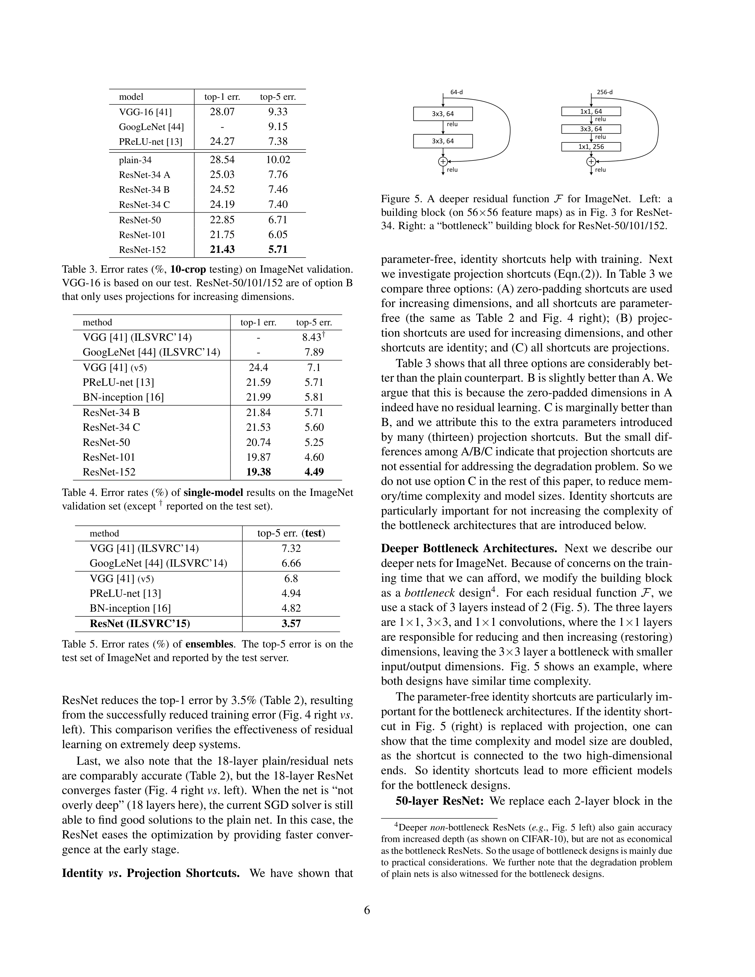
Figure 4. Training on
ImageNet
.
Thin curves denote training error, and bold curves denote validation error of the center crops.
Left:
plain
networks of 18 and 34 layers.
Right:
ResNets of 18 and 34 layers.
In this plot, the residual networks have no extra parameter compared to
their plain counterparts.
plain
ResNet
18 layers
27.94
27.88
34 layers
28.54
25.03
Table 2. Top-1 error (%, 10-crop testing) on ImageNet validation.
Here the ResNets have no extra parameter compared to their plain
counterparts.
Fig. 4 shows the training procedures.
34-layer
plain
net
has
higher
training
error
throughout
the
whole
training
procedure,
even
though
the
solution
space
of
the
18-layer
plain
network
is
a
subspace
of
that
of
the
34-layer one.
We
argue
that
this
optimization
difficulty
is
unlikely
to
be caused by vanishing gradients.
These plain networks are
trained
with
BN
[16],
which
ensures
forward
propagated
signals to have non-zero variances.
We also verify that the
backward propagated gradients exhibit healthy norms with
BN.
So
neither
forward
nor
backward
signals
vanish.
In
fact,
the
34-layer
plain
net
is
still
able
to
achieve
compet-
itive
accuracy
(Table
3),
suggesting
that
the
solver
works
to some extent.
We conjecture that the deep plain nets may
have exponentially low convergence rates, which impact the
reducing
of
the
training
error
3
.
The
reason
for
such
opti-
mization difficulties will be studied in the future.
Residual
Networks.
Next
we
evaluate
18-layer
and
34-
layer
residual
nets
(
ResNets
).
The
baseline
architectures
are the same as the above plain nets, expect that a shortcut
connection is added to each pair of 3
×
3 filters as in Fig. 3
(right).
In
the
first
comparison
(Table
2
and
Fig.
4
right),
we use identity mapping for all shortcuts and zero-padding
for increasing dimensions (option A). So they have
no extra
parameter
compared to the plain counterparts.
We
have
three
major
observations
from
Table
2
and
Fig.
4.
First,
the
situation
is
reversed
with
residual
learn-
ing – the 34-layer ResNet is better than the 18-layer ResNet
(by 2.8%).
More importantly, the 34-layer ResNet exhibits
considerably lower training error and is generalizable to the
validation data.
This indicates that the degradation problem
is
well
addressed
in
this
setting
and
we
manage
to
obtain
accuracy gains from increased depth.
Second,
compared
to
its
plain
counterpart,
the
34-layer
3
We have experimented with more training iterations (3
×
) and still ob-
served
the
degradation
problem,
suggesting
that
this
problem
cannot
be
feasibly addressed by simply using more iterations.
5
model
top-1 err.
top-5 err.
VGG-16 [41]
28.07
9.33
GoogLeNet [44]
-
9.15
PReLU-net [13]
24.27
7.38
plain-34
28.54
10.02
ResNet-34 A
25.03
7.76
ResNet-34 B
24.52
7.46
ResNet-34 C
24.19
7.40
ResNet-50
22.85
6.71
ResNet-101
21.75
6.05
ResNet-152
21.43
5.71
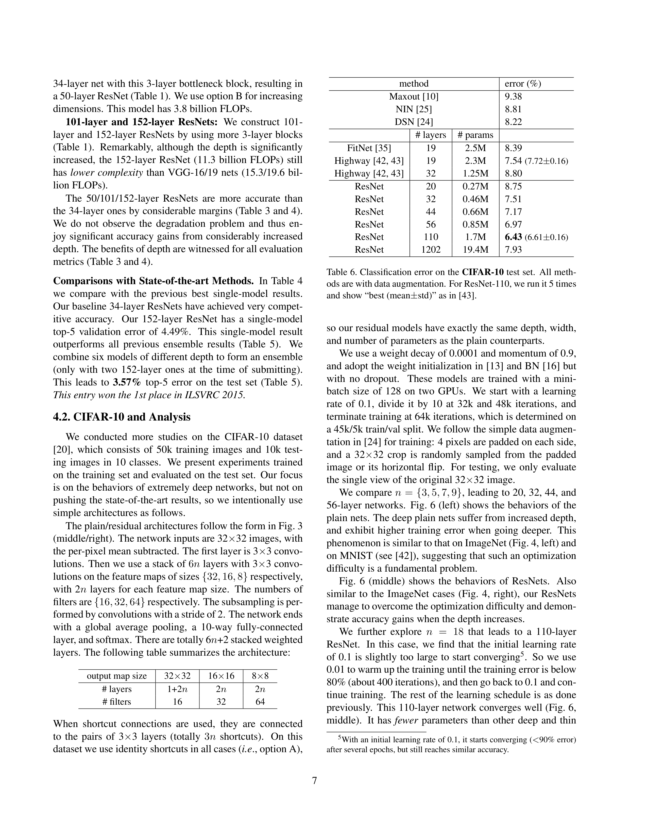
Table 3. Error rates (%,
10-crop
testing) on ImageNet validation.
VGG-16 is based on our test.
ResNet-50/101/152 are of option B
that only uses projections for increasing dimensions.
method
top-1 err.
top-5 err.
VGG [41] (ILSVRC’14)
-
8.43
†
GoogLeNet [44] (ILSVRC’14)
-
7.89
VGG [41]
(v5)
24.4
7.1
PReLU-net [13]
21.59
5.71
BN-inception [16]
21.99
5.81
ResNet-34 B
21.84
5.71
ResNet-34 C
21.53
5.60
ResNet-50
20.74
5.25
ResNet-101
19.87
4.60
ResNet-152
19.38
4.49
Table 4. Error rates (%) of
single-model
results on the ImageNet
validation set (except
†
reported on the test set).
method
top-5 err.
(
test
)
VGG [41] (ILSVRC’14)
7.32
GoogLeNet [44] (ILSVRC’14)
6.66
VGG [41]
(v5)
6.8
PReLU-net [13]
4.94
BN-inception [16]
4.82
ResNet (ILSVRC’15)
3.57
Table
5.
Error
rates
(%)
of
ensembles
.
The
top-5
error
is
on
the
test set of ImageNet and reported by the test server.
ResNet reduces the top-1 error by 3.5% (Table 2), resulting
from the successfully reduced training error (Fig. 4 right
vs
.
left).
This comparison verifies the effectiveness of residual
learning on extremely deep systems.
Last,
we
also
note
that
the
18-layer
plain/residual
nets
are comparably accurate (Table 2), but the 18-layer ResNet
converges faster (Fig. 4 right
vs
. left).
When the net is “not
overly deep” (18 layers here), the current SGD solver is still
able to find good solutions to the plain net.
In this case, the
ResNet
eases
the
optimization
by
providing
faster
conver-
gence at the early stage.
Identity
vs
.
Projection
Shortcuts.
We
have
shown
that
3x3, 64
1x1, 64
relu
1x1, 256
relu
relu
3x3, 64
3x3, 64
relu
relu
64-d
256-d
Figure
5.
A
deeper
residual
function
F
for
ImageNet.
Left:
a
building
block
(on
56
×
56
feature
maps)
as
in
Fig.
3
for
ResNet-
34.
Right:
a “bottleneck” building block for ResNet-50/101/152.
parameter-free,
identity
shortcuts
help
with
training.
Next
we investigate projection shortcuts (Eqn.(2)).
In Table 3 we
compare three options:
(A) zero-padding shortcuts are used
for increasing dimensions,
and all shortcuts are parameter-
free
(the
same
as
Table
2
and
Fig.
4
right);
(B)
projec-
tion shortcuts are used for increasing dimensions, and other
shortcuts are identity; and (C) all shortcuts are projections.
Table 3 shows that all three options are considerably bet-
ter than the plain counterpart. B is slightly better than A. We
argue that this is because the zero-padded dimensions in A
indeed have no residual learning. C is marginally better than
B,
and
we
attribute
this
to
the
extra
parameters
introduced
by
many
(thirteen)
projection
shortcuts.
But
the
small
dif-
ferences among A/B/C indicate that projection shortcuts are
not essential for addressing the degradation problem. So we
do not use option C in the rest of this paper, to reduce mem-
ory/time complexity and model sizes.
Identity shortcuts are
particularly
important
for
not
increasing
the
complexity
of
the bottleneck architectures that are introduced below.
Deeper
Bottleneck
Architectures.
Next
we
describe
our
deeper nets for ImageNet. Because of concerns on the train-
ing
time
that
we
can
afford,
we
modify
the
building
block
as
a
bottleneck
design
4
.
For
each
residual
function
F
,
we
use a stack of 3 layers instead of 2 (Fig. 5).
The three layers
are 1
×
1, 3
×
3, and 1
×
1 convolutions, where the 1
×
1 layers
are responsible for reducing and then increasing (restoring)
dimensions, leaving the 3
×
3 layer a bottleneck with smaller
input/output
dimensions.
Fig.
5
shows
an
example,
where
both designs have similar time complexity.
The parameter-free identity shortcuts are particularly im-
portant for the bottleneck architectures. If the identity short-
cut
in
Fig.
5
(right)
is
replaced
with
projection,
one
can
show that the time complexity and model size are doubled,
as
the
shortcut
is
connected
to
the
two
high-dimensional
ends.
So
identity
shortcuts
lead
to
more
efficient
models
for the bottleneck designs.
50-layer
ResNet:
We
replace
each
2-layer
block
in
the
4
Deeper
non
-bottleneck
ResNets
(
e.g
.,
Fig.
5
left)
also
gain
accuracy
from increased depth (as shown on CIFAR-10), but are not as economical
as the bottleneck ResNets. So the usage of bottleneck designs is mainly due
to
practical
considerations.
We
further
note
that
the
degradation
problem
of plain nets is also witnessed for the bottleneck designs.
6
34-layer net with this 3-layer bottleneck block, resulting in
a 50-layer ResNet (Table 1). We use option B for increasing
dimensions.
This model has 3.8 billion FLOPs.
101-layer
and
152-layer
ResNets:
We
construct
101-
layer
and
152-layer
ResNets
by
using
more
3-layer
blocks
(Table
1).
Remarkably,
although
the
depth
is
significantly
increased,
the
152-layer
ResNet
(11.3
billion
FLOPs)
still
has
lower
complexity
than
VGG-16/19
nets
(15.3/19.6
bil-
lion FLOPs).
The
50/101/152-layer
ResNets
are
more
accurate
than
the 34-layer ones by considerable margins (Table 3 and 4).
We
do
not
observe
the
degradation
problem
and
thus
en-
joy
significant
accuracy
gains
from
considerably
increased
depth.
The benefits of depth are witnessed for all evaluation
metrics (Table 3 and 4).
Comparisons
with
State-of-the-art
Methods.
In
Table
4
we
compare
with
the
previous
best
single-model
results.
Our baseline 34-layer ResNets have achieved very compet-
itive
accuracy.
Our
152-layer
ResNet
has
a
single-model
top-5
validation
error
of
4.49%.
This
single-model
result
outperforms
all
previous
ensemble
results
(Table
5).
We
combine six models of different depth to form an ensemble
(only
with
two
152-layer
ones
at
the
time
of
submitting).
This
leads
to
3.57%
top-5
error
on
the
test
set
(Table
5).
This entry won the 1st place in ILSVRC 2015.
4.2. CIFAR-10 and Analysis
We
conducted
more
studies
on
the
CIFAR-10
dataset
[20],
which
consists
of
50k
training
images
and
10k
test-
ing
images
in
10
classes.
We
present
experiments
trained
on the training set and evaluated on the test set.
Our focus
is on the behaviors of extremely deep networks, but not on
pushing the state-of-the-art results,
so we intentionally use
simple architectures as follows.
The plain/residual architectures follow the form in Fig. 3
(middle/right).
The network inputs are 32
×
32 images, with
the per-pixel mean subtracted.
The first layer is 3
×
3 convo-
lutions.
Then we use a stack of
6
n
layers with 3
×
3 convo-
lutions on the feature maps of sizes
{
32
,
16
,
8
}
respectively,
with
2
n
layers
for
each
feature
map
size.
The
numbers
of
filters are
{
16
,
32
,
64
}
respectively. The subsampling is per-
formed by convolutions with a stride of 2. The network ends
with
a
global
average
pooling,
a
10-way
fully-connected
layer, and softmax. There are totally 6
n
+2 stacked weighted
layers.
The following table summarizes the architecture:
output map size
32
×
32
16
×
16
8
×
8
# layers
1+2
n
2
n
2
n
# filters
16
32
64
When
shortcut
connections
are
used,
they
are
connected
to
the
pairs
of
3
×
3
layers
(totally
3
n
shortcuts).
On
this
dataset we use identity shortcuts in all cases (
i.e
., option A),
method
error (%)
Maxout [10]
9.38
NIN [25]
8.81
DSN [24]
8.22
# layers
# params
FitNet [35]
19
2.5M
8.39
Highway [42, 43]
19
2.3M
7.54
(7.72
±
0.16)
Highway [42, 43]
32
1.25M
8.80
ResNet
20
0.27M
8.75
ResNet
32
0.46M
7.51
ResNet
44
0.66M
7.17
ResNet
56
0.85M
6.97
ResNet
110
1.7M
6.43
(6.61
±
0.16)
ResNet
1202
19.4M
7.93
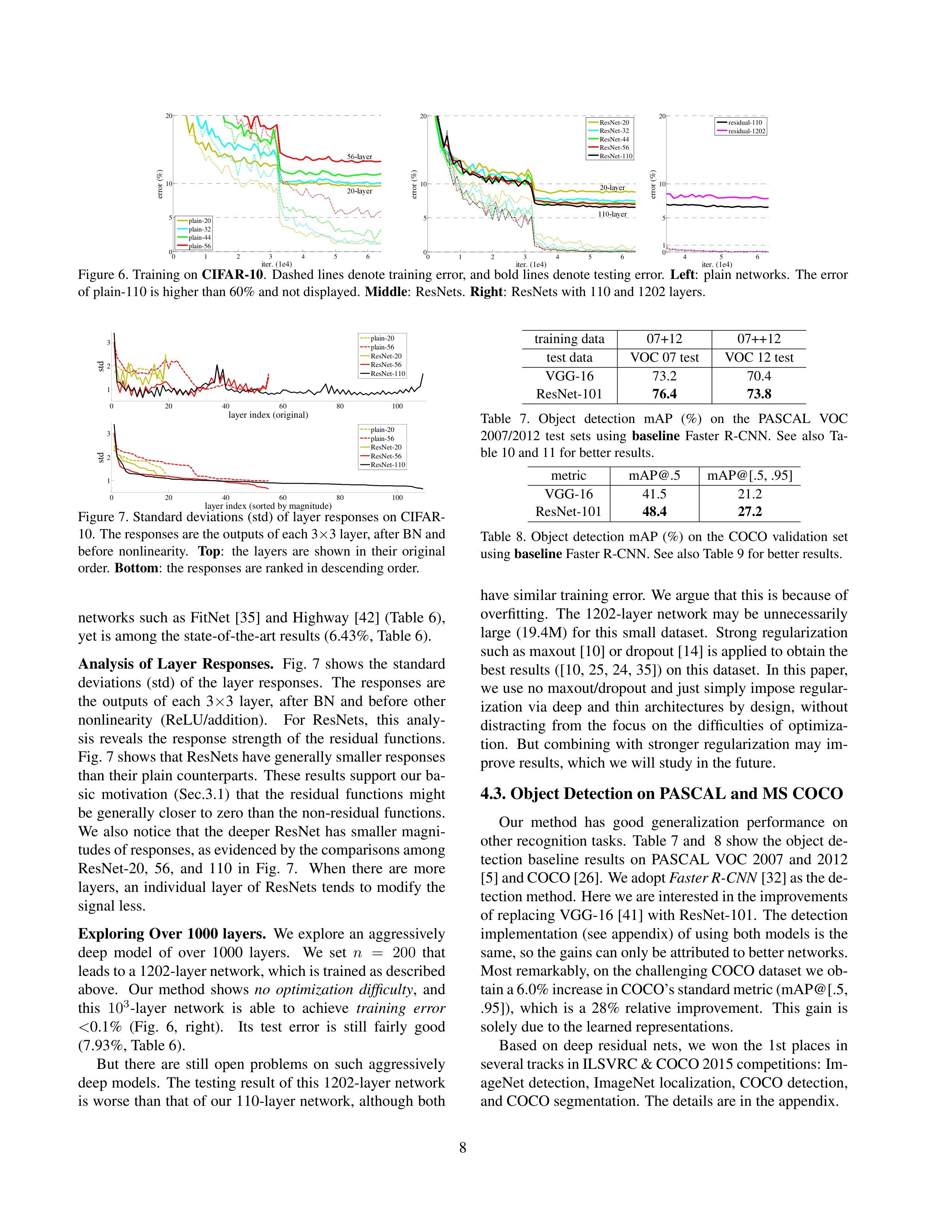
Table 6. Classification error on the
CIFAR-10
test set.
All meth-
ods are with data augmentation. For ResNet-110, we run it 5 times
and show “best (mean
±
std)” as in [43].
so our residual models have exactly the same depth, width,
and number of parameters as the plain counterparts.
We use a weight decay of 0.0001 and momentum of 0.9,
and adopt the weight initialization in [13] and BN [16] but
with
no
dropout.
These
models
are
trained
with
a
mini-
batch
size
of
128
on
two
GPUs.
We
start
with
a
learning
rate
of
0.1,
divide
it
by
10
at
32k
and
48k
iterations,
and
terminate training at 64k iterations, which is determined on
a 45k/5k train/val split.
We follow the simple data augmen-
tation in [24] for training:
4 pixels are padded on each side,
and
a
32
×
32
crop
is
randomly
sampled
from
the
padded
image
or
its
horizontal
flip.
For
testing,
we
only
evaluate
the single view of the original 32
×
32 image.
We compare
n
=
{
3
,
5
,
7
,
9
}
, leading to 20, 32, 44, and
56-layer networks.
Fig. 6 (left) shows the behaviors of the
plain nets.
The deep plain nets suffer from increased depth,
and
exhibit
higher
training
error
when
going
deeper.
This
phenomenon is similar to that on ImageNet (Fig. 4, left) and
on MNIST (see [42]), suggesting that such an optimization
difficulty is a fundamental problem.
Fig.
6
(middle)
shows
the
behaviors
of
ResNets.
Also
similar
to
the
ImageNet
cases
(Fig.
4,
right),
our
ResNets
manage to overcome the optimization difficulty and demon-
strate accuracy gains when the depth increases.
We
further
explore
n
=
18
that
leads
to
a
110-layer
ResNet.
In
this
case,
we
find
that
the
initial
learning
rate
of
0.1
is
slightly
too
large
to
start
converging
5
.
So
we
use
0.01 to warm up the training until the training error is below
80% (about 400 iterations), and then go back to 0.1 and con-
tinue training.
The rest of the learning schedule is as done
previously.
This 110-layer network converges well (Fig. 6,
middle).
It
has
fewer
parameters
than
other
deep
and
thin
5
With an initial learning rate of 0.1, it starts converging (
<
90% error)
after several epochs, but still reaches similar accuracy.
7
0
1
2
3
4
5
6
0
5
10
20
iter. (1e4)
error (%)
plain-20
plain-32
plain-44
plain-56
0
1
2
3
4
5
6
0
5
10
20
iter. (1e4)
error (%)
ResNet-20
ResNet-32
ResNet-44
ResNet-56
ResNet-110
56-layer
20-layer
110-layer
20-layer
4
5
6
0
1
5
10
20
iter. (1e4)
error (%)
residual-110
residual-1202
Figure 6. Training on
CIFAR-10
.
Dashed lines denote training error, and bold lines denote testing error.
Left
:
plain networks.
The error
of plain-110 is higher than 60% and not displayed.
Middle
:
ResNets.
Right
:
ResNets with 110 and 1202 layers.
0
20
40
60
80
100
1
2
3
layer index (sorted by magnitude)
std
plain-20
plain-56
ResNet-20
ResNet-56
ResNet-110
0
20
40
60
80
100
1
2
3
layer index (original)
std
plain-20
plain-56
ResNet-20
ResNet-56
ResNet-110
Figure 7. Standard deviations (std) of layer responses on CIFAR-
10.
The responses are the outputs of each 3
×
3 layer, after BN and
before
nonlinearity.
Top
:
the
layers
are
shown
in
their
original
order.
Bottom
:
the responses are ranked in descending order.
networks
such
as
FitNet
[35]
and
Highway
[42]
(Table
6),
yet is among the state-of-the-art results (6.43%, Table 6).
Analysis
of
Layer
Responses.
Fig.
7
shows
the
standard
deviations
(std)
of
the
layer
responses.
The
responses
are
the
outputs
of
each
3
×
3
layer,
after
BN
and
before
other
nonlinearity
(ReLU/addition).
For
ResNets,
this
analy-
sis
reveals
the
response
strength
of
the
residual
functions.
Fig. 7 shows that ResNets have generally smaller responses
than their plain counterparts.
These results support our ba-
sic
motivation
(Sec.3.1)
that
the
residual
functions
might
be generally closer to zero than the non-residual functions.
We
also
notice
that
the
deeper
ResNet
has
smaller
magni-
tudes of responses, as evidenced by the comparisons among
ResNet-20,
56,
and
110
in
Fig.
7.
When
there
are
more
layers,
an
individual
layer
of
ResNets
tends
to
modify
the
signal less.
Exploring
Over
1000
layers.
We
explore
an
aggressively
deep
model
of
over
1000
layers.
We
set
n
=
200
that
leads to a 1202-layer network, which is trained as described
above.
Our
method
shows
no
optimization
difficulty
,
and
this
10
3
-layer
network
is
able
to
achieve
training
error
<
0.1%
(Fig.
6,
right).
Its
test
error
is
still
fairly
good
(7.93%, Table 6).
But
there
are
still
open
problems
on
such
aggressively
deep models.
The testing result of this 1202-layer network
is worse than that of our 110-layer network,
although both
training data
07+12
07++12
test data
VOC 07 test
VOC 12 test
VGG-16
73.2
70.4
ResNet-101
76.4
73.8
Table
7.
Object
detection
mAP
(%)
on
the
PASCAL
VOC
2007/2012
test
sets
using
baseline
Faster
R-CNN.
See
also
Ta-
ble 10 and 11 for better results.
metric
mAP@.5
mAP@[.5, .95]
VGG-16
41.5
21.2
ResNet-101
48.4
27.2
Table
8.
Object
detection
mAP
(%)
on
the
COCO
validation
set
using
baseline
Faster R-CNN. See also Table 9 for better results.
have similar training error.
We argue that this is because of
overfitting.
The
1202-layer
network
may
be
unnecessarily
large
(19.4M)
for
this
small
dataset.
Strong
regularization
such as maxout [10] or dropout [14] is applied to obtain the
best results ([10, 25, 24, 35]) on this dataset.
In this paper,
we use no maxout/dropout and just simply impose regular-
ization
via
deep
and
thin
architectures
by
design,
without
distracting
from
the
focus
on
the
difficulties
of
optimiza-
tion.
But
combining
with
stronger
regularization
may
im-
prove results, which we will study in the future.
4.3. Object Detection on PASCAL and MS COCO
Our
method
has
good
generalization
performance
on
other recognition tasks.
Table 7 and
8 show the object de-
tection
baseline
results
on
PASCAL
VOC
2007
and
2012
[5] and COCO [26]. We adopt
Faster R-CNN
[32] as the de-
tection method. Here we are interested in the improvements
of replacing VGG-16 [41] with ResNet-101.
The detection
implementation (see appendix) of using both models is the
same, so the gains can only be attributed to better networks.
Most remarkably, on the challenging COCO dataset we ob-
tain a 6.0% increase in COCO’s standard metric (mAP@[.5,
.95]),
which
is
a
28%
relative
improvement.
This
gain
is
solely due to the learned representations.
Based
on
deep
residual
nets,
we
won
the
1st
places
in
several tracks in ILSVRC & COCO 2015 competitions: Im-
ageNet detection, ImageNet localization, COCO detection,
and COCO segmentation.
The details are in the appendix.
8
References
[1]
Y. Bengio, P. Simard, and P. Frasconi. Learning long-term dependen-
cies with gradient descent is difficult.
IEEE Transactions on Neural
Networks
, 5(2):157–166, 1994.
[2]
C.
M.
Bishop.
Neural
networks
for
pattern
recognition
.
Oxford
university press, 1995.
[3]
W.
L.
Briggs,
S.
F.
McCormick,
et
al.
A
Multigrid
Tutorial
.
Siam,
2000.
[4]
K. Chatfield, V. Lempitsky, A. Vedaldi, and A. Zisserman.
The devil
is
in
the
details:
an
evaluation
of
recent
feature
encoding
methods.
In
BMVC
, 2011.
[5]
M. Everingham,
L. Van Gool,
C. K. Williams,
J. Winn,
and A. Zis-
serman.
The Pascal Visual Object Classes (VOC) Challenge.
IJCV
,
pages 303–338, 2010.
[6]
S. Gidaris and N. Komodakis.
Object detection via a multi-region &
semantic segmentation-aware cnn model.
In
ICCV
, 2015.
[7]
R. Girshick.
Fast R-CNN.
In
ICCV
, 2015.
[8]
R. Girshick, J. Donahue, T. Darrell, and J. Malik.
Rich feature hier-
archies for accurate object detection and semantic segmentation.
In
CVPR
, 2014.
[9]
X.
Glorot
and
Y.
Bengio.
Understanding
the
difficulty
of
training
deep feedforward neural networks.
In
AISTATS
, 2010.
[10]
I.
J.
Goodfellow,
D.
Warde-Farley,
M.
Mirza,
A.
Courville,
and
Y. Bengio.
Maxout networks.
arXiv:1302.4389
, 2013.
[11]
K. He and J. Sun.
Convolutional neural networks at constrained time
cost.
In
CVPR
, 2015.
[12]
K. He, X. Zhang, S. Ren, and J. Sun. Spatial pyramid pooling in deep
convolutional networks for visual recognition.
In
ECCV
, 2014.
[13]
K.
He,
X.
Zhang,
S.
Ren,
and
J.
Sun.
Delving
deep
into
rectifiers:
Surpassing human-level performance on imagenet classification.
In
ICCV
, 2015.
[14]
G.
E.
Hinton,
N.
Srivastava,
A.
Krizhevsky,
I.
Sutskever,
and
R.
R.
Salakhutdinov.
Improving
neural
networks
by
preventing
co-
adaptation of feature detectors.
arXiv:1207.0580
, 2012.
[15]
S. Hochreiter and J. Schmidhuber.
Long short-term memory.
Neural
computation
, 9(8):1735–1780, 1997.
[16]
S.
Ioffe
and
C.
Szegedy.
Batch
normalization:
Accelerating
deep
network training by reducing internal covariate shift. In
ICML
, 2015.
[17]
H. Jegou, M. Douze, and C. Schmid. Product quantization for nearest
neighbor search.
TPAMI
, 33, 2011.
[18]
H.
Jegou,
F.
Perronnin,
M.
Douze,
J.
Sanchez,
P.
Perez,
and
C. Schmid.
Aggregating local image descriptors into compact codes.
TPAMI
, 2012.
[19]
Y. Jia,
E. Shelhamer,
J. Donahue,
S. Karayev,
J. Long,
R. Girshick,
S. Guadarrama, and T. Darrell.
Caffe:
Convolutional architecture for
fast feature embedding.
arXiv:1408.5093
, 2014.
[20]
A.
Krizhevsky.
Learning
multiple
layers
of
features
from
tiny
im-
ages.
Tech Report
, 2009.
[21]
A. Krizhevsky,
I. Sutskever,
and G. Hinton.
Imagenet classification
with deep convolutional neural networks.
In
NIPS
, 2012.
[22]
Y.
LeCun,
B.
Boser,
J.
S.
Denker,
D.
Henderson,
R.
E.
Howard,
W.
Hubbard,
and
L.
D.
Jackel.
Backpropagation
applied
to
hand-
written zip code recognition.
Neural computation
, 1989.
[23]
Y. LeCun, L. Bottou, G. B. Orr, and K.-R. M¨uller. Efficient backprop.
In
Neural Networks: Tricks of the Trade
, pages 9–50. Springer, 1998.
[24]
C.-Y.
Lee,
S.
Xie,
P.
Gallagher,
Z.
Zhang,
and
Z.
Tu.
Deeply-
supervised nets.
arXiv:1409.5185
, 2014.
[25]
M. Lin, Q. Chen, and S. Yan. Network in network.
arXiv:1312.4400
,
2013.
[26]
T.-Y.
Lin,
M.
Maire,
S.
Belongie,
J.
Hays,
P.
Perona,
D.
Ramanan,
P. Doll´ar,
and C. L. Zitnick.
Microsoft COCO: Common objects in
context.
In
ECCV
. 2014.
[27]
J. Long, E. Shelhamer, and T. Darrell.
Fully convolutional networks
for semantic segmentation.
In
CVPR
, 2015.
[28]
G. Mont´ufar, R. Pascanu, K. Cho, and Y. Bengio.
On the number of
linear regions of deep neural networks.
In
NIPS
, 2014.
[29]
V.
Nair
and
G.
E.
Hinton.
Rectified
linear
units
improve
restricted
boltzmann machines.
In
ICML
, 2010.
[30]
F. Perronnin and C. Dance.
Fisher kernels on visual vocabularies for
image categorization.
In
CVPR
, 2007.
[31]
T. Raiko,
H. Valpola,
and Y. LeCun.
Deep learning made easier by
linear transformations in perceptrons.
In
AISTATS
, 2012.
[32]
S.
Ren,
K.
He,
R.
Girshick,
and
J.
Sun.
Faster
R-CNN:
Towards
real-time
object
detection
with
region
proposal
networks.
In
NIPS
,
2015.
[33]
S. Ren, K. He, R. Girshick, X. Zhang, and J. Sun.
Object detection
networks on convolutional feature maps.
arXiv:1504.06066
, 2015.
[34]
B. D. Ripley.
Pattern recognition and neural networks
.
Cambridge
university press, 1996.
[35]
A.
Romero,
N.
Ballas,
S.
E.
Kahou,
A.
Chassang,
C.
Gatta,
and
Y. Bengio.
Fitnets:
Hints for thin deep nets.
In
ICLR
, 2015.
[36]
O.
Russakovsky,
J.
Deng,
H.
Su,
J.
Krause,
S.
Satheesh,
S.
Ma,
Z.
Huang,
A.
Karpathy,
A.
Khosla,
M.
Bernstein,
et
al.
Imagenet
large scale visual recognition challenge.
arXiv:1409.0575
, 2014.
[37]
A.
M.
Saxe,
J.
L.
McClelland,
and
S.
Ganguli.
Exact
solutions
to
the
nonlinear
dynamics
of
learning
in
deep
linear
neural
networks.
arXiv:1312.6120
, 2013.
[38]
N. N. Schraudolph.
Accelerated gradient descent by factor-centering
decomposition.
Technical report, 1998.
[39]
N.
N.
Schraudolph.
Centering
neural
network
gradient
factors.
In
Neural
Networks:
Tricks
of
the
Trade
,
pages
207–226.
Springer,
1998.
[40]
P. Sermanet, D. Eigen, X. Zhang, M. Mathieu, R. Fergus, and Y. Le-
Cun.
Overfeat:
Integrated
recognition,
localization
and
detection
using convolutional networks.
In
ICLR
, 2014.
[41]
K.
Simonyan
and
A.
Zisserman.
Very
deep
convolutional
networks
for large-scale image recognition.
In
ICLR
, 2015.
[42]
R. K. Srivastava, K. Greff, and J. Schmidhuber.
Highway networks.
arXiv:1505.00387
, 2015.
[43]
R. K. Srivastava, K. Greff, and J. Schmidhuber.
Training very deep
networks.
1507.06228
, 2015.
[44]
C. Szegedy, W. Liu, Y. Jia, P. Sermanet, S. Reed, D. Anguelov, D. Er-
han, V. Vanhoucke, and A. Rabinovich.
Going deeper with convolu-
tions.
In
CVPR
, 2015.
[45]
R. Szeliski.
Fast surface interpolation using hierarchical basis func-
tions.
TPAMI
, 1990.
[46]
R.
Szeliski.
Locally
adapted
hierarchical
basis
preconditioning.
In
SIGGRAPH
, 2006.
[47]
T.
Vatanen,
T.
Raiko,
H.
Valpola,
and
Y.
LeCun.
Pushing
stochas-
tic
gradient
towards
second-order
methods–backpropagation
learn-
ing
with
transformations
in
nonlinearities.
In
Neural
Information
Processing
, 2013.
[48]
A. Vedaldi and B. Fulkerson.
VLFeat:
An open and portable library
of computer vision algorithms, 2008.
[49]
W.
Venables
and
B.
Ripley.
Modern
applied
statistics
with
s-plus.
1999.
[50]
M. D. Zeiler and R. Fergus.
Visualizing and understanding convolu-
tional neural networks.
In
ECCV
, 2014.
9
A. Object Detection Baselines
In this section we introduce our detection method based
on the baseline Faster R-CNN [32] system.
The models are
initialized by the ImageNet classification models, and then
fine-tuned
on
the
object
detection
data.
We
have
experi-
mented
with
ResNet-50/101
at
the
time
of
the
ILSVRC
&
COCO 2015 detection competitions.
Unlike VGG-16 used in [32], our ResNet has no hidden
fc
layers.
We
adopt
the
idea
of
“Networks
on
Conv
fea-
ture
maps”
(NoC)
[33]
to
address
this
issue.
We
compute
the
full-image
shared
conv
feature
maps
using
those
lay-
ers whose strides on the image are no greater than 16 pixels
(
i.e
., conv1, conv2
x, conv3
x, and conv4
x, totally 91 conv
layers in ResNet-101; Table 1).
We consider these layers as
analogous
to
the
13
conv
layers
in
VGG-16,
and
by
doing
so, both ResNet and VGG-16 have conv feature maps of the
same
total
stride
(16
pixels).
These
layers
are
shared
by
a
region
proposal
network
(RPN,
generating
300
proposals)
[32]
and
a
Fast
R-CNN
detection
network
[7].
RoI
pool-
ing
[7]
is
performed
before
conv5
1.
On
this
RoI-pooled
feature,
all
layers
of
conv5
x
and
up
are
adopted
for
each
region,
playing
the
roles
of
VGG-16’s
fc
layers.
The
final
classification layer is replaced by two sibling layers (classi-
fication and box regression [7]).
For
the
usage
of
BN
layers,
after
pre-training,
we
com-
pute the BN statistics (means and variances) for each layer
on the ImageNet training set.
Then the BN layers are fixed
during
fine-tuning
for
object
detection.
As
such,
the
BN
layers
become
linear
activations
with
constant
offsets
and
scales, and BN statistics are not updated by fine-tuning.
We
fix the BN layers mainly for reducing memory consumption
in Faster R-CNN training.
PASCAL VOC
Following
[7,
32],
for
the
PASCAL
VOC
2007
test
set,
we use the 5k
trainval
images in VOC 2007 and 16k
train-
val
images
in
VOC
2012
for
training
(“07+12”).
For
the
PASCAL
VOC
2012
test
set,
we
use
the
10k
trainval
+
test
images in VOC 2007 and 16k
trainval
images in VOC 2012
for
training
(“07++12”).
The
hyper-parameters
for
train-
ing
Faster
R-CNN
are
the
same
as
in
[32].
Table
7
shows
the
results.
ResNet-101
improves
the
mAP
by
>
3%
over
VGG-16.
This gain is solely
because of the improved fea-
tures learned by ResNet.
MS COCO
The
MS
COCO
dataset
[26]
involves
80
object
cate-
gories.
We
evaluate
the
PASCAL
VOC
metric
(mAP
@
IoU = 0.5) and the standard COCO metric (mAP @ IoU =
.5:.05:.95).
We use the 80k images on the train set for train-
ing
and
the
40k
images
on
the
val
set
for
evaluation.
Our
detection system for COCO
is similar to
that for
PASCAL
VOC.
We
train
the
COCO
models
with
an
8-GPU
imple-
mentation,
and
thus
the
RPN
step
has
a
mini-batch
size
of
8
images
(
i.e
.,
1
per
GPU)
and
the
Fast
R-CNN
step
has
a
mini-batch
size
of
16
images.
The
RPN
step
and
Fast
R-
CNN step are both trained for 240k iterations with a learn-
ing rate of 0.001 and then for 80k iterations with 0.0001.
Table
8
shows
the
results
on
the
MS
COCO
validation
set.
ResNet-101 has a 6% increase of mAP@[.5, .95] over
VGG-16, which is a 28% relative improvement, solely con-
tributed by the features learned by the better network.
Re-
markably, the mAP@[.5, .95]’s absolute increase (6.0%) is
nearly
as
big
as
mAP@.5’s
(6.9%).
This
suggests
that
a
deeper network can improve both recognition and localiza-
tion.
B. Object Detection Improvements
For completeness, we report the improvements made for
the
competitions.
These
improvements
are
based
on
deep
features and thus should benefit from residual learning.
MS COCO
Box refinement.
Our box refinement partially follows the it-
erative localization in [6]. In Faster R-CNN, the final output
is a regressed box that is different from its proposal box.
So
for inference, we pool a new feature from the regressed box
and
obtain
a
new
classification
score
and
a
new
regressed
box.
We combine these 300 new predictions with the orig-
inal 300 predictions.
Non-maximum suppression (NMS) is
applied
on
the
union
set
of
predicted
boxes
using
an
IoU
threshold
of
0.3
[8],
followed
by
box
voting
[6].
Box
re-
finement improves mAP by about 2 points (Table 9).
Global
context.
We
combine
global
context
in
the
Fast
R-CNN
step.
Given
the
full-image
conv
feature
map,
we
pool a feature by global Spatial Pyramid Pooling [12] (with
a
“single-level”
pyramid)
which
can
be
implemented
as
“RoI” pooling using the entire image’s bounding box as the
RoI.
This
pooled
feature
is
fed
into
the
post-RoI
layers
to
obtain a global context feature.
This global feature is con-
catenated
with
the
original
per-region
feature,
followed
by
the
sibling
classification
and
box
regression
layers.
This
new
structure
is
trained
end-to-end.
Global
context
im-
proves mAP@.5 by about 1 point (Table 9).
Multi-scale testing.
In the above, all results are obtained by
single-scale
training/testing
as
in
[32],
where
the
image’s
shorter side is
s
=
600
pixels.
Multi-scale training/testing
has
been
developed
in
[12,
7]
by
selecting
a
scale
from
a
feature
pyramid,
and
in
[33]
by
using
maxout
layers.
In
our current implementation, we have performed multi-scale
testing
following
[33];
we
have
not
performed
multi-scale
training because of limited time.
In addition,
we have per-
formed
multi-scale
testing
only
for
the
Fast
R-CNN
step
(but
not
yet
for
the
RPN
step).
With
a
trained
model,
we
compute conv feature maps on an image pyramid, where the
image’s
shorter
sides
are
s
∈{
200
,
400
,
600
,
800
,
1000
}
.
10
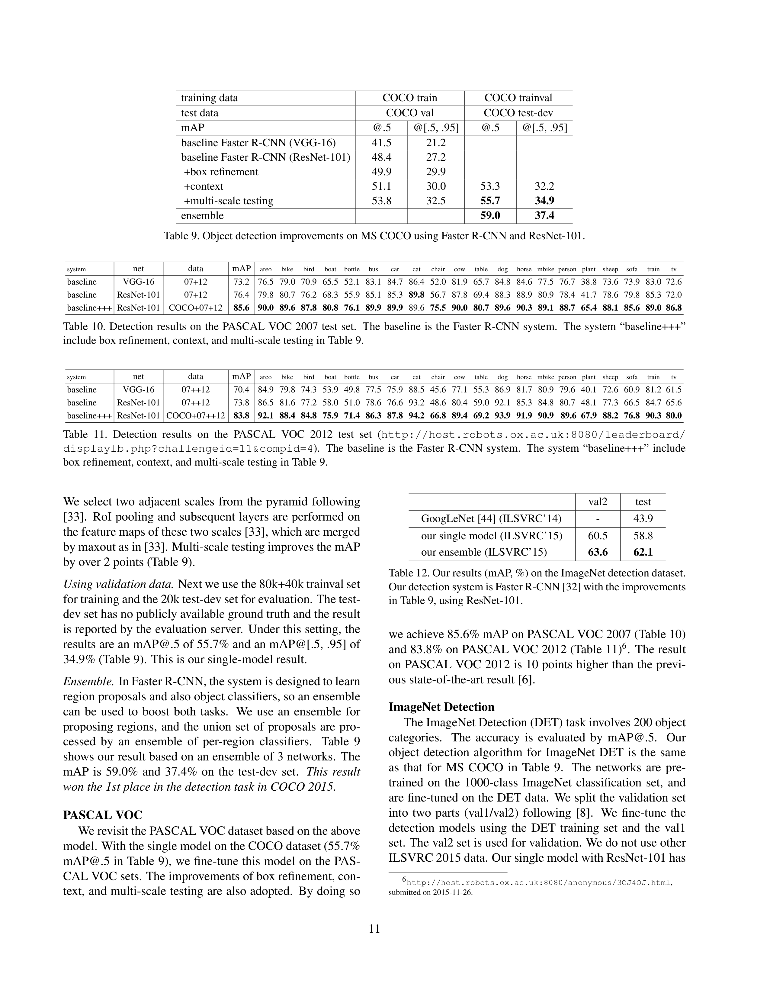
training data
COCO train
COCO trainval
test data
COCO val
COCO test-dev
mAP
@.5
@[.5, .95]
@.5
@[.5, .95]
baseline Faster R-CNN (VGG-16)
41.5
21.2
baseline Faster R-CNN (ResNet-101)
48.4
27.2
+box refinement
49.9
29.9
+context
51.1
30.0
53.3
32.2
+multi-scale testing
53.8
32.5
55.7
34.9
ensemble
59.0
37.4
Table 9. Object detection improvements on MS COCO using Faster R-CNN and ResNet-101.
system
net
data
mAP
areo
bike
bird
boat
bottle
bus
car
cat
chair
cow
table
dog
horse
mbike
person
plant
sheep
sofa
train
tv
baseline
VGG-16
07+12
73.2
76.5
79.0
70.9
65.5
52.1
83.1
84.7
86.4
52.0
81.9
65.7
84.8
84.6
77.5
76.7
38.8
73.6
73.9
83.0
72.6
baseline
ResNet-101
07+12
76.4
79.8
80.7
76.2
68.3
55.9
85.1
85.3
89.8
56.7
87.8
69.4
88.3
88.9
80.9
78.4
41.7
78.6
79.8
85.3
72.0
baseline+++
ResNet-101
COCO+07+12
85.6
90.0
89.6
87.8
80.8
76.1
89.9
89.9
89.6
75.5
90.0
80.7
89.6
90.3
89.1
88.7
65.4
88.1
85.6
89.0
86.8
Table
10.
Detection
results
on
the
PASCAL
VOC
2007
test
set.
The
baseline
is
the
Faster
R-CNN
system.
The
system
“baseline+++”
include box refinement, context, and multi-scale testing in Table 9.
system
net
data
mAP
areo
bike
bird
boat
bottle
bus
car
cat
chair
cow
table
dog
horse
mbike
person
plant
sheep
sofa
train
tv
baseline
VGG-16
07++12
70.4
84.9
79.8
74.3
53.9
49.8
77.5
75.9
88.5
45.6
77.1
55.3
86.9
81.7
80.9
79.6
40.1
72.6
60.9
81.2
61.5
baseline
ResNet-101
07++12
73.8
86.5
81.6
77.2
58.0
51.0
78.6
76.6
93.2
48.6
80.4
59.0
92.1
85.3
84.8
80.7
48.1
77.3
66.5
84.7
65.6
baseline+++
ResNet-101
COCO+07++12
83.8
92.1
88.4
84.8
75.9
71.4
86.3
87.8
94.2
66.8
89.4
69.2
93.9
91.9
90.9
89.6
67.9
88.2
76.8
90.3
80.0
Table
11.
Detection
results
on
the
PASCAL
VOC
2012
test
set
(
http://host.robots.ox.ac.uk:8080/leaderboard/
displaylb.php?challengeid=11&compid=4
).
The
baseline
is
the
Faster
R-CNN
system.
The
system
“baseline+++”
include
box refinement, context, and multi-scale testing in Table 9.
We
select
two
adjacent
scales
from
the
pyramid
following
[33].
RoI
pooling
and
subsequent
layers
are
performed
on
the feature maps of these two scales [33], which are merged
by maxout as in [33]. Multi-scale testing improves the mAP
by over 2 points (Table 9).
Using validation data.
Next we use the 80k+40k trainval set
for training and the 20k test-dev set for evaluation. The test-
dev set has no publicly available ground truth and the result
is reported by the evaluation server.
Under this setting, the
results are an mAP@.5 of 55.7% and an mAP@[.5, .95] of
34.9% (Table 9).
This is our single-model result.
Ensemble.
In Faster R-CNN, the system is designed to learn
region proposals and also object classifiers, so an ensemble
can
be
used
to
boost
both
tasks.
We
use
an
ensemble
for
proposing
regions,
and
the
union
set
of
proposals
are
pro-
cessed
by
an
ensemble
of
per-region
classifiers.
Table
9
shows our result based on an ensemble of 3 networks.
The
mAP
is
59.0%
and
37.4%
on
the
test-dev
set.
This
result
won the 1st place in the detection task in COCO 2015.
PASCAL VOC
We revisit the PASCAL VOC dataset based on the above
model.
With the single model on the COCO dataset (55.7%
mAP@.5 in Table 9),
we fine-tune this model on the PAS-
CAL VOC sets.
The improvements of box refinement, con-
text,
and multi-scale testing are also adopted.
By doing so
val2
test
GoogLeNet [44] (ILSVRC’14)
-
43.9
our single model (ILSVRC’15)
60.5
58.8
our ensemble (ILSVRC’15)
63.6
62.1
Table 12. Our results (mAP, %) on the ImageNet detection dataset.
Our detection system is Faster R-CNN [32] with the improvements
in Table 9, using ResNet-101.
we achieve 85.6% mAP on PASCAL VOC 2007 (Table 10)
and 83.8% on PASCAL VOC 2012 (Table 11)
6
.
The result
on PASCAL VOC 2012 is 10 points higher than the previ-
ous state-of-the-art result [6].
ImageNet Detection
The ImageNet Detection (DET) task involves 200 object
categories.
The
accuracy
is
evaluated
by
mAP@.5.
Our
object
detection
algorithm
for
ImageNet
DET
is
the
same
as
that
for
MS
COCO
in
Table
9.
The
networks
are
pre-
trained
on
the
1000-class
ImageNet
classification
set,
and
are fine-tuned on the DET data.
We split the validation set
into
two
parts
(val1/val2)
following
[8].
We
fine-tune
the
detection
models
using
the
DET
training
set
and
the
val1
set.
The val2 set is used for validation.
We do not use other
ILSVRC 2015 data.
Our single model with ResNet-101 has
6
http://host.robots.ox.ac.uk:8080/anonymous/3OJ4OJ.html
,
submitted on 2015-11-26.
11
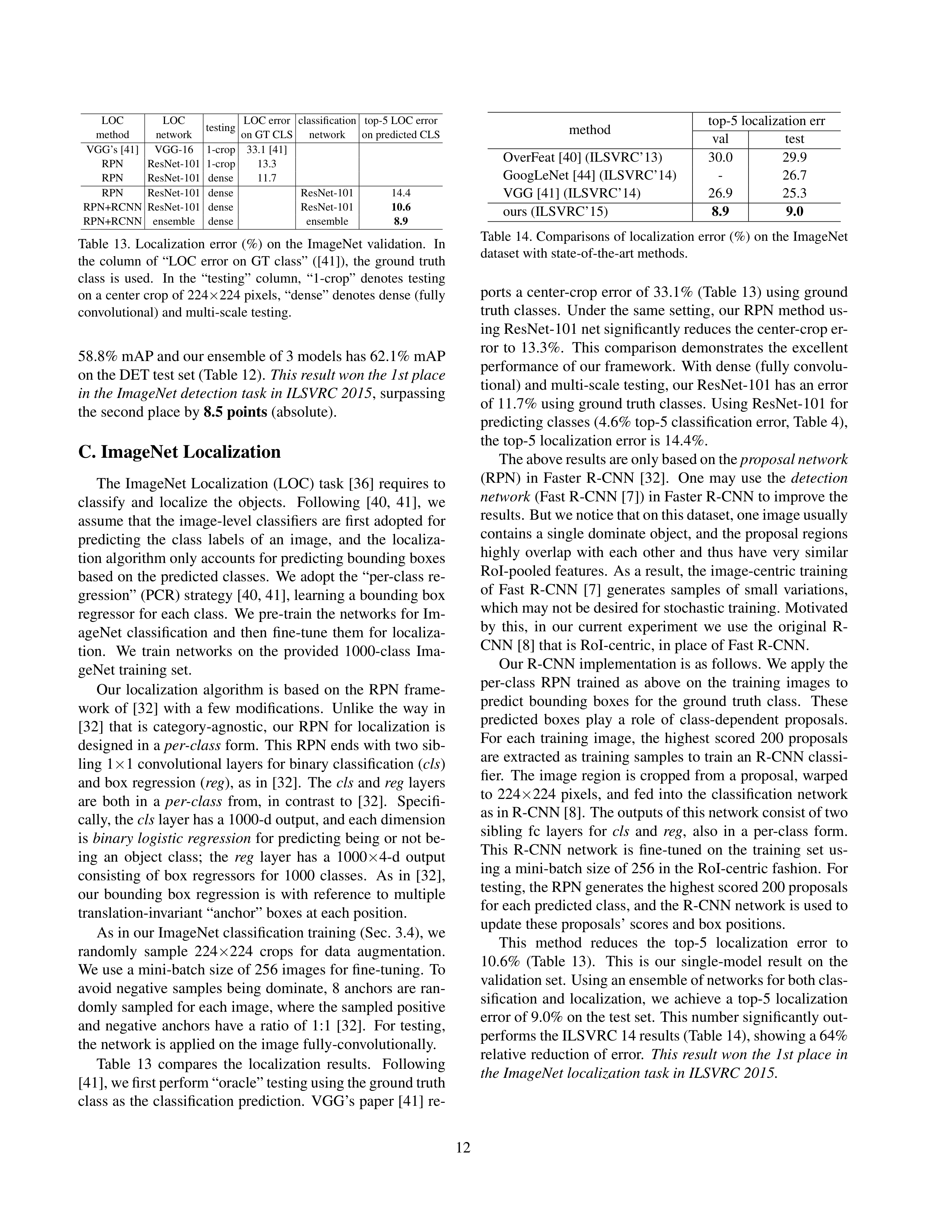
LOC
method
LOC
network
testing
LOC error
on GT CLS
classification
network
top-5 LOC error
on predicted CLS
VGG’s [41]
VGG-16
1-crop
33.1 [41]
RPN
ResNet-101
1-crop
13.3
RPN
ResNet-101
dense
11.7
RPN
ResNet-101
dense
ResNet-101
14.4
RPN+RCNN
ResNet-101
dense
ResNet-101
10.6
RPN+RCNN
ensemble
dense
ensemble
8.9
Table
13.
Localization
error
(%)
on
the
ImageNet
validation.
In
the
column
of
“LOC
error
on
GT
class”
([41]),
the
ground
truth
class
is
used.
In
the
“testing”
column,
“1-crop”
denotes
testing
on a center crop of 224
×
224 pixels, “dense” denotes dense (fully
convolutional) and multi-scale testing.
58.8% mAP and our ensemble of 3 models has 62.1% mAP
on the DET test set (Table 12).
This result won the 1st place
in the ImageNet detection task in ILSVRC 2015
, surpassing
the second place by
8.5 points
(absolute).
C. ImageNet Localization
The ImageNet Localization (LOC) task [36] requires to
classify
and
localize
the
objects.
Following
[40,
41],
we
assume that the image-level classifiers are first adopted for
predicting
the
class
labels
of
an
image,
and
the
localiza-
tion algorithm only accounts for predicting bounding boxes
based on the predicted classes.
We adopt the “per-class re-
gression” (PCR) strategy [40, 41], learning a bounding box
regressor for each class.
We pre-train the networks for Im-
ageNet
classification
and
then
fine-tune
them
for
localiza-
tion.
We
train
networks
on
the
provided
1000-class
Ima-
geNet training set.
Our
localization
algorithm
is
based
on
the
RPN
frame-
work
of
[32]
with
a
few
modifications.
Unlike
the
way
in
[32]
that
is
category-agnostic,
our
RPN
for
localization
is
designed in a
per-class
form.
This RPN ends with two sib-
ling 1
×
1 convolutional layers for binary classification (
cls
)
and box regression (
reg
), as in [32].
The
cls
and
reg
layers
are
both
in
a
per-class
from,
in
contrast
to
[32].
Specifi-
cally, the
cls
layer has a 1000-d output, and each dimension
is
binary logistic regression
for predicting being or not be-
ing
an
object
class;
the
reg
layer
has
a
1000
×
4-d
output
consisting
of
box
regressors
for
1000
classes.
As
in
[32],
our
bounding
box
regression
is
with
reference
to
multiple
translation-invariant “anchor” boxes at each position.
As in our ImageNet classification training (Sec. 3.4), we
randomly
sample
224
×
224
crops
for
data
augmentation.
We use a mini-batch size of 256 images for fine-tuning.
To
avoid negative samples being dominate,
8 anchors are ran-
domly sampled for each image, where the sampled positive
and
negative
anchors
have
a
ratio
of
1:1
[32].
For
testing,
the network is applied on the image fully-convolutionally.
Table
13
compares
the
localization
results.
Following
[41], we first perform “oracle” testing using the ground truth
class as the classification prediction.
VGG’s paper [41] re-
method
top-5 localization err
val
test
OverFeat [40] (ILSVRC’13)
30.0
29.9
GoogLeNet [44] (ILSVRC’14)
-
26.7
VGG [41] (ILSVRC’14)
26.9
25.3
ours (ILSVRC’15)
8.9
9.0
Table 14. Comparisons of localization error (%) on the ImageNet
dataset with state-of-the-art methods.
ports a center-crop error of 33.1% (Table 13) using ground
truth classes.
Under the same setting, our RPN method us-
ing ResNet-101 net significantly reduces the center-crop er-
ror
to
13.3%.
This
comparison
demonstrates
the
excellent
performance of our framework.
With dense (fully convolu-
tional) and multi-scale testing, our ResNet-101 has an error
of 11.7% using ground truth classes.
Using ResNet-101 for
predicting classes (4.6% top-5 classification error, Table 4),
the top-5 localization error is 14.4%.
The above results are only based on the
proposal network
(RPN)
in
Faster
R-CNN
[32].
One
may
use
the
detection
network
(Fast R-CNN [7]) in Faster R-CNN to improve the
results. But we notice that on this dataset, one image usually
contains a single dominate object, and the proposal regions
highly
overlap
with
each
other
and
thus
have
very
similar
RoI-pooled features.
As a result, the image-centric training
of
Fast
R-CNN
[7]
generates
samples
of
small
variations,
which may not be desired for stochastic training.
Motivated
by
this,
in
our
current
experiment
we
use
the
original
R-
CNN [8] that is RoI-centric, in place of Fast R-CNN.
Our R-CNN implementation is as follows.
We apply the
per-class
RPN
trained
as
above
on
the
training
images
to
predict
bounding
boxes
for
the
ground
truth
class.
These
predicted
boxes
play
a
role
of
class-dependent
proposals.
For
each
training
image,
the
highest
scored
200
proposals
are extracted as training samples to train an R-CNN classi-
fier.
The image region is cropped from a proposal, warped
to
224
×
224
pixels,
and
fed
into
the
classification
network
as in R-CNN [8]. The outputs of this network consist of two
sibling
fc
layers
for
cls
and
reg
,
also
in
a
per-class
form.
This
R-CNN
network
is
fine-tuned
on
the
training
set
us-
ing a mini-batch size of 256 in the RoI-centric fashion.
For
testing, the RPN generates the highest scored 200 proposals
for each predicted class, and the R-CNN network is used to
update these proposals’ scores and box positions.
This
method
reduces
the
top-5
localization
error
to
10.6%
(Table
13).
This
is
our
single-model
result
on
the
validation set. Using an ensemble of networks for both clas-
sification
and
localization,
we
achieve
a
top-5
localization
error of 9.0% on the test set.
This number significantly out-
performs the ILSVRC 14 results (Table 14), showing a 64%
relative reduction of error.
This result won the 1st place in
the ImageNet localization task in ILSVRC 2015.
12