Pixel Recurrent Neural Networks
A¨aron van den Oord
AVDNOORD
@
GOOGLE
.
COM
Nal Kalchbrenner
NALK
@
GOOGLE
.
COM
Koray Kavukcuoglu
KORAYK
@
GOOGLE
.
COM
Google DeepMind
Abstract
Modeling
the
distribution
of
natural
images
is
a
landmark
problem
in
unsupervised
learning.
This
task
requires
an
image
model
that
is
at
once
expressive,
tractable
and
scalable.
We
present
a
deep
neural
network
that
sequentially
predicts
the
pixels
in
an
image
along
the
two
spatial dimensions.
Our method models the dis-
crete probability of the raw pixel values and en-
codes
the
complete
set
of
dependencies
in
the
image.
Architectural
novelties
include
fast
two-
dimensional recurrent layers and an effective use
of
residual
connections
in
deep
recurrent
net-
works.
We achieve log-likelihood scores on nat-
ural images that are considerably better than the
previous
state
of
the
art.
Our
main
results
also
provide
benchmarks
on
the
diverse
ImageNet
dataset.
Samples
generated
from
the
model
ap-
pear crisp, varied and globally coherent.
1. Introduction
Generative
image
modeling
is
a
central
problem
in
unsu-
pervised learning. Probabilistic density models can be used
for a wide variety of tasks that range from image compres-
sion and forms of reconstruction such as image inpainting
(e.g.,
see
Figure
1
)
and
deblurring,
to
generation
of
new
images.
When the model is conditioned on external infor-
mation, possible applications also include creating images
based on text descriptions or simulating future frames in a
planning
task.
One
of
the
great
advantages
in
generative
modeling
is
that
there
are
practically
endless
amounts
of
image data available to learn from.
However,
because im-
ages are high dimensional and highly structured, estimating
the distribution of natural images is extremely challenging.
One
of
the
most
important
obstacles
in
generative
mod-
Proceedings
of
the
33
rd
International
Conference
on
Machine
Learning
,
New
York,
NY,
USA,
2016.
JMLR:
W&CP
volume
48.
Copyright 2016 by the author(s).
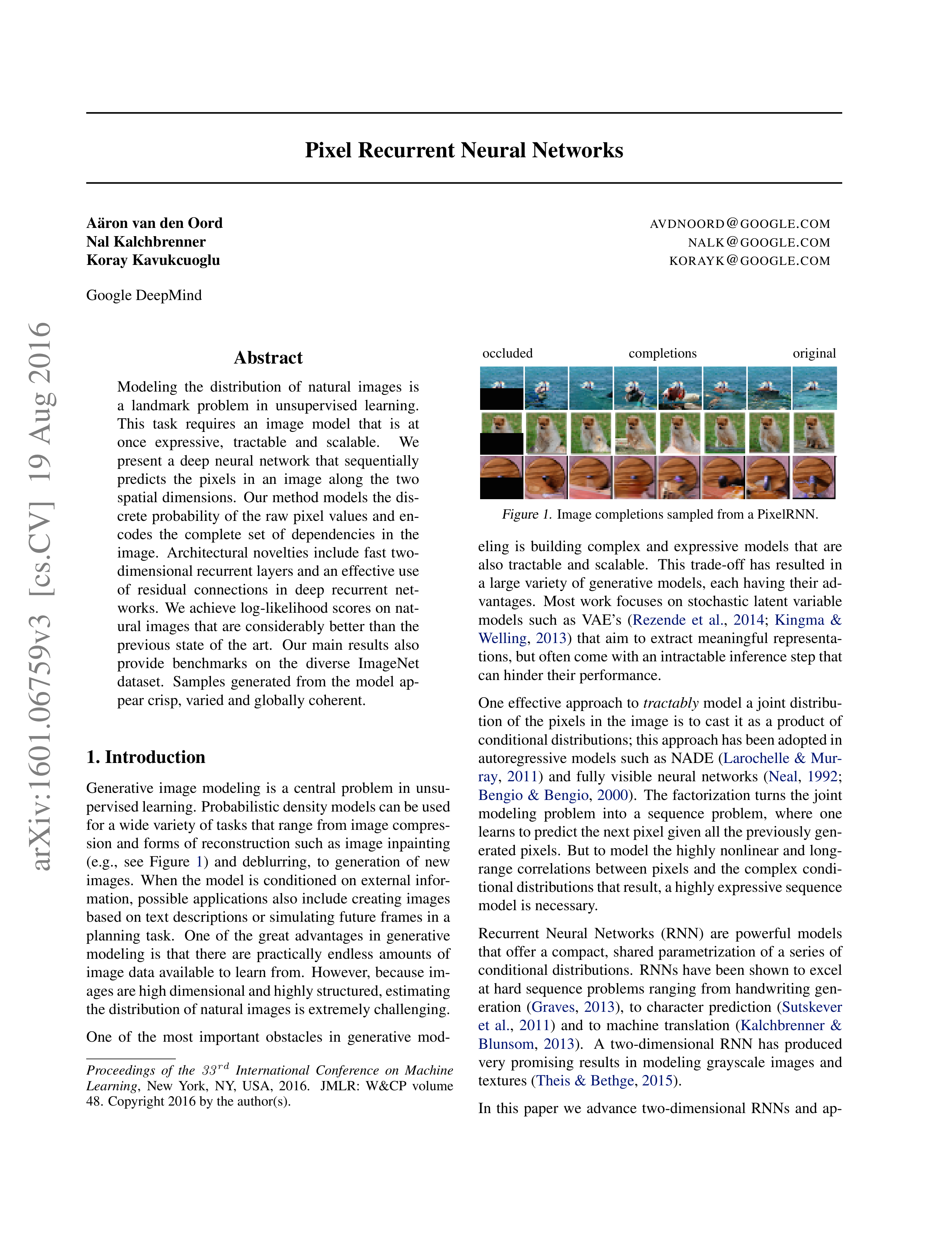
occluded
completions
original
Figure 1.
Image completions sampled from a PixelRNN.
eling
is
building
complex
and
expressive
models
that
are
also
tractable
and
scalable.
This
trade-off
has
resulted
in
a large variety of generative models, each having their ad-
vantages.
Most
work
focuses
on
stochastic
latent
variable
models
such
as
VAE’s
(
Rezende
et
al.
,
2014
;
Kingma
&
Welling
,
2013
)
that
aim
to
extract
meaningful
representa-
tions, but often come with an intractable inference step that
can hinder their performance.
One effective approach to
tractably
model a joint distribu-
tion
of
the
pixels
in
the
image
is
to
cast
it
as
a
product
of
conditional distributions; this approach has been adopted in
autoregressive models such as NADE (
Larochelle & Mur-
ray
,
2011
)
and
fully
visible
neural
networks
(
Neal
,
1992
;
Bengio & Bengio
,
2000
).
The factorization turns the joint
modeling
problem
into
a
sequence
problem,
where
one
learns to predict the next pixel given all the previously gen-
erated pixels.
But to model the highly nonlinear and long-
range
correlations
between
pixels
and
the
complex
condi-
tional distributions that result, a highly expressive sequence
model is necessary.
Recurrent
Neural
Networks
(RNN)
are
powerful
models
that offer
a compact,
shared parametrization of a
series of
conditional distributions.
RNNs have been shown to excel
at hard sequence problems ranging from handwriting gen-
eration
(
Graves
,
2013
),
to
character
prediction
(
Sutskever
et
al.
,
2011
)
and
to
machine
translation
(
Kalchbrenner
&
Blunsom
,
2013
).
A
two-dimensional
RNN
has
produced
very
promising
results
in
modeling
grayscale
images
and
textures (
Theis & Bethge
,
2015
).
In
this
paper
we
advance
two-dimensional
RNNs
and
ap-
arXiv:1601.06759v3 [cs.CV] 19 Aug 2016
Pixel Recurrent Neural Networks
x
1
x
i
x
n
x
n
2
Context
x
n
2
Multi-scale context
x
1
x
i
x
n
x
n
2
R
G
B
R
G
B
R
G
B
Mask
A
Mask
B
Context
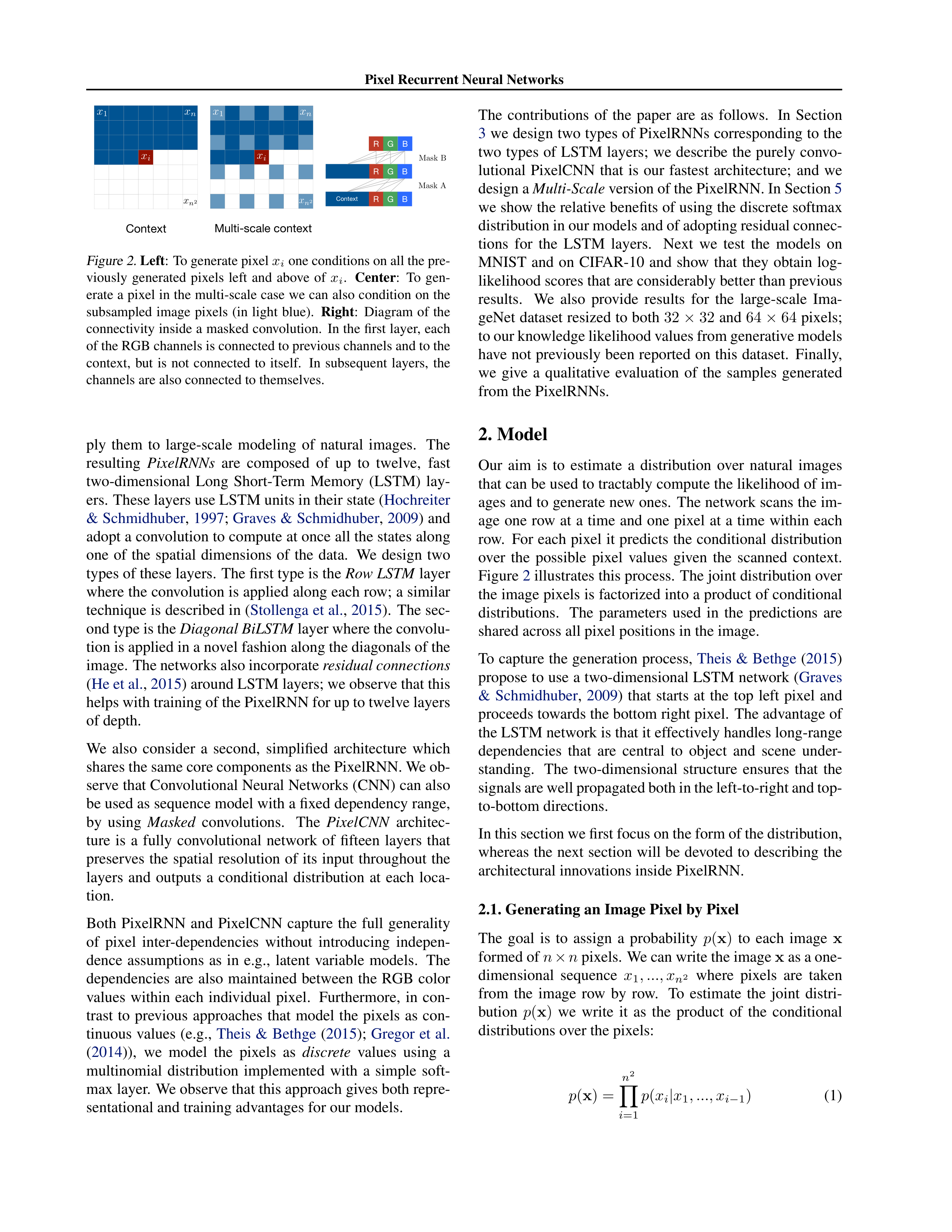
Figure 2.
Left
:
To generate pixel
x
i
one conditions on all the pre-
viously
generated
pixels
left
and
above
of
x
i
.
Center
:
To
gen-
erate a pixel in the multi-scale case we can also condition on the
subsampled
image
pixels
(in
light
blue).
Right
:
Diagram
of
the
connectivity inside a masked convolution.
In the first layer, each
of the RGB channels is connected to previous channels and to the
context,
but
is
not
connected
to
itself.
In
subsequent
layers,
the
channels are also connected to themselves.
ply
them
to
large-scale
modeling
of
natural
images.
The
resulting
PixelRNNs
are
composed
of
up
to
twelve,
fast
two-dimensional
Long
Short-Term
Memory
(LSTM)
lay-
ers.
These layers use LSTM units in their state (
Hochreiter
& Schmidhuber
,
1997
;
Graves & Schmidhuber
,
2009
) and
adopt a convolution to compute at once all the states along
one
of
the
spatial
dimensions
of
the
data.
We
design
two
types of these layers.
The first type is the
Row LSTM
layer
where the convolution is applied along each row; a similar
technique is described in (
Stollenga et al.
,
2015
).
The sec-
ond type is the
Diagonal BiLSTM
layer where the convolu-
tion is applied in a novel fashion along the diagonals of the
image. The networks also incorporate
residual connections
(
He et al.
,
2015
) around LSTM layers; we observe that this
helps with training of the PixelRNN for up to twelve layers
of depth.
We
also
consider
a
second,
simplified
architecture
which
shares the same core components as the PixelRNN. We ob-
serve that Convolutional Neural Networks (CNN) can also
be used as sequence model with a fixed dependency range,
by
using
Masked
convolutions.
The
PixelCNN
architec-
ture
is
a
fully
convolutional
network
of
fifteen
layers
that
preserves
the
spatial
resolution
of
its
input
throughout
the
layers
and
outputs
a
conditional
distribution
at
each
loca-
tion.
Both
PixelRNN
and
PixelCNN
capture
the
full
generality
of
pixel
inter-dependencies
without
introducing
indepen-
dence
assumptions
as
in
e.g.,
latent
variable
models.
The
dependencies
are
also
maintained
between
the
RGB
color
values
within
each
individual
pixel.
Furthermore,
in
con-
trast
to
previous
approaches
that
model
the
pixels
as
con-
tinuous values (e.g.,
Theis & Bethge
(
2015
);
Gregor et al.
(
2014
)),
we
model
the
pixels
as
discrete
values
using
a
multinomial
distribution
implemented
with
a
simple
soft-
max layer.
We observe that this approach gives both repre-
sentational and training advantages for our models.
The
contributions
of
the
paper
are
as
follows.
In
Section
3
we design two types of PixelRNNs corresponding to the
two types
of LSTM
layers;
we
describe the purely
convo-
lutional
PixelCNN
that
is
our
fastest
architecture;
and
we
design a
Multi-Scale
version of the PixelRNN. In Section
5
we show the relative benefits of using the discrete softmax
distribution in our models and of adopting residual connec-
tions
for
the
LSTM
layers.
Next
we
test
the
models
on
MNIST
and
on
CIFAR-10
and
show
that
they
obtain
log-
likelihood scores that are considerably better than previous
results.
We
also
provide
results
for
the
large-scale
Ima-
geNet dataset resized to both
32
×
32
and
64
×
64
pixels;
to our knowledge likelihood values from generative models
have not previously been reported on this dataset.
Finally,
we
give
a
qualitative
evaluation
of
the
samples
generated
from the PixelRNNs.
2. Model
Our
aim
is
to
estimate
a
distribution
over
natural
images
that can be used to tractably compute the likelihood of im-
ages and to generate new ones.
The network scans the im-
age
one
row
at
a
time
and
one
pixel
at
a
time
within
each
row.
For each pixel it predicts the conditional distribution
over
the
possible
pixel
values
given
the
scanned
context.
Figure
2
illustrates this process.
The joint distribution over
the image pixels is factorized into a product of conditional
distributions.
The
parameters
used
in
the
predictions
are
shared across all pixel positions in the image.
To capture the generation process,
Theis & Bethge
(
2015
)
propose to use a two-dimensional LSTM network (
Graves
&
Schmidhuber
,
2009
)
that
starts
at
the
top
left
pixel
and
proceeds towards the bottom right pixel.
The advantage of
the LSTM network is that it effectively handles long-range
dependencies
that
are
central
to
object
and
scene
under-
standing.
The
two-dimensional
structure
ensures
that
the
signals are well propagated both in the left-to-right and top-
to-bottom directions.
In this section we first focus on the form of the distribution,
whereas the next section will be devoted to describing the
architectural innovations inside PixelRNN.
2.1. Generating an Image Pixel by Pixel
The
goal
is
to
assign
a
probability
p
(
x
)
to
each
image
x
formed of
n
×
n
pixels.
We can write the image
x
as a one-
dimensional
sequence
x
1
, ..., x
n
2
where
pixels
are
taken
from
the
image
row
by
row.
To
estimate
the
joint
distri-
bution
p
(
x
)
we
write
it
as
the
product
of
the
conditional
distributions over the pixels:
p
(
x
) =
n
2
Y
i
=1
p
(
x
i
|
x
1
, ..., x
i
−
1
)
(1)
Pixel Recurrent Neural Networks
The
value
p
(
x
i
|
x
1
, ..., x
i
−
1
)
is
the
probability
of
the
i
-th
pixel
x
i
given all the previous pixels
x
1
, ..., x
i
−
1
.
The gen-
eration
proceeds
row
by
row
and
pixel
by
pixel.
Figure
2
(Left) illustrates the conditioning scheme.
Each pixel
x
i
is in turn jointly determined by three values,
one
for
each
of
the
color
channels
Red,
Green
and
Blue
(RGB).
We
rewrite
the
distribution
p
(
x
i
|
x
<i
)
as
the
fol-
lowing product:
p
(
x
i,R
|
x
<i
)
p
(
x
i,G
|
x
<i
, x
i,R
)
p
(
x
i,B
|
x
<i
, x
i,R
, x
i,G
)
(2)
Each of the colors is thus conditioned on the other channels
as well as on all the previously generated pixels.
Note
that
during
training
and
evaluation
the
distributions
over
the
pixel
values
are
computed
in
parallel
,
while
the
generation of an image is
sequential
.
2.2. Pixels as Discrete Variables
Previous
approaches
use
a
continuous
distribution
for
the
values
of
the
pixels
in
the
image
(e.g.
Theis
&
Bethge
(
2015
);
Uria et al.
(
2014
)).
By contrast we model
p
(
x
)
as
a
discrete
distribution,
with
every
conditional
distribution
in
Equation
2
being
a
multinomial
that
is
modeled
with
a
softmax layer.
Each channel variable
x
i,
∗
simply takes one
of 256 distinct values. The discrete distribution is represen-
tationally simple and has the advantage of being arbitrarily
multimodal without prior on the shape (see Fig.
6
).
Exper-
imentally
we
also
find
the
discrete
distribution
to
be
easy
to
learn
and
to
produce
better
performance
compared
to
a
continuous distribution (Section
5
).
3. Pixel Recurrent Neural Networks
In
this
section
we
describe
the
architectural
components
that
compose
the
PixelRNN.
In
Sections
3.1
and
3.2
,
we
describe
the
two
types
of
LSTM
layers
that
use
convolu-
tions to compute at once the states along one of the spatial
dimensions.
In Section
3.3
we describe how to incorporate
residual
connections to improve the training of a PixelRNN
with
many
LSTM
layers.
In
Section
3.4
we
describe
the
softmax
layer
that
computes
the
discrete
joint
distribution
of
the
colors
and
the
masking
technique
that
ensures
the
proper conditioning scheme. In Section
3.5
we describe the
PixelCNN architecture.
Finally in Section
3.6
we describe
the multi-scale architecture.
3.1. Row LSTM
The
Row
LSTM
is
a
unidirectional
layer
that
processes
the
image
row
by
row
from
top
to
bottom
computing
fea-
tures
for
a
whole
row
at
once;
the
computation
is
per-
formed
with
a
one-dimensional
convolution.
For
a
pixel
x
i
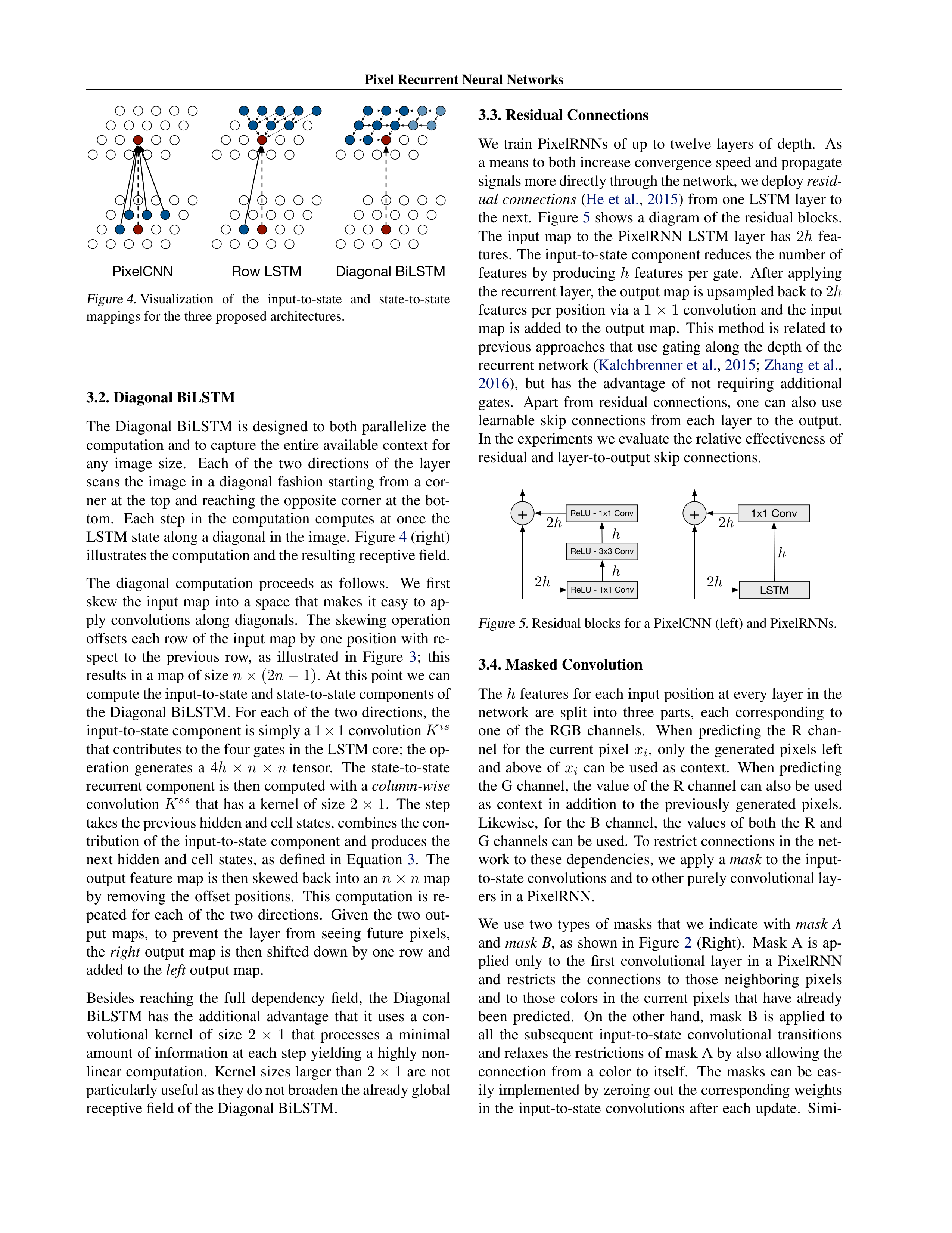
the layer captures a roughly triangular context above the
pixel as shown in Figure
4
(center).
The kernel of the one-
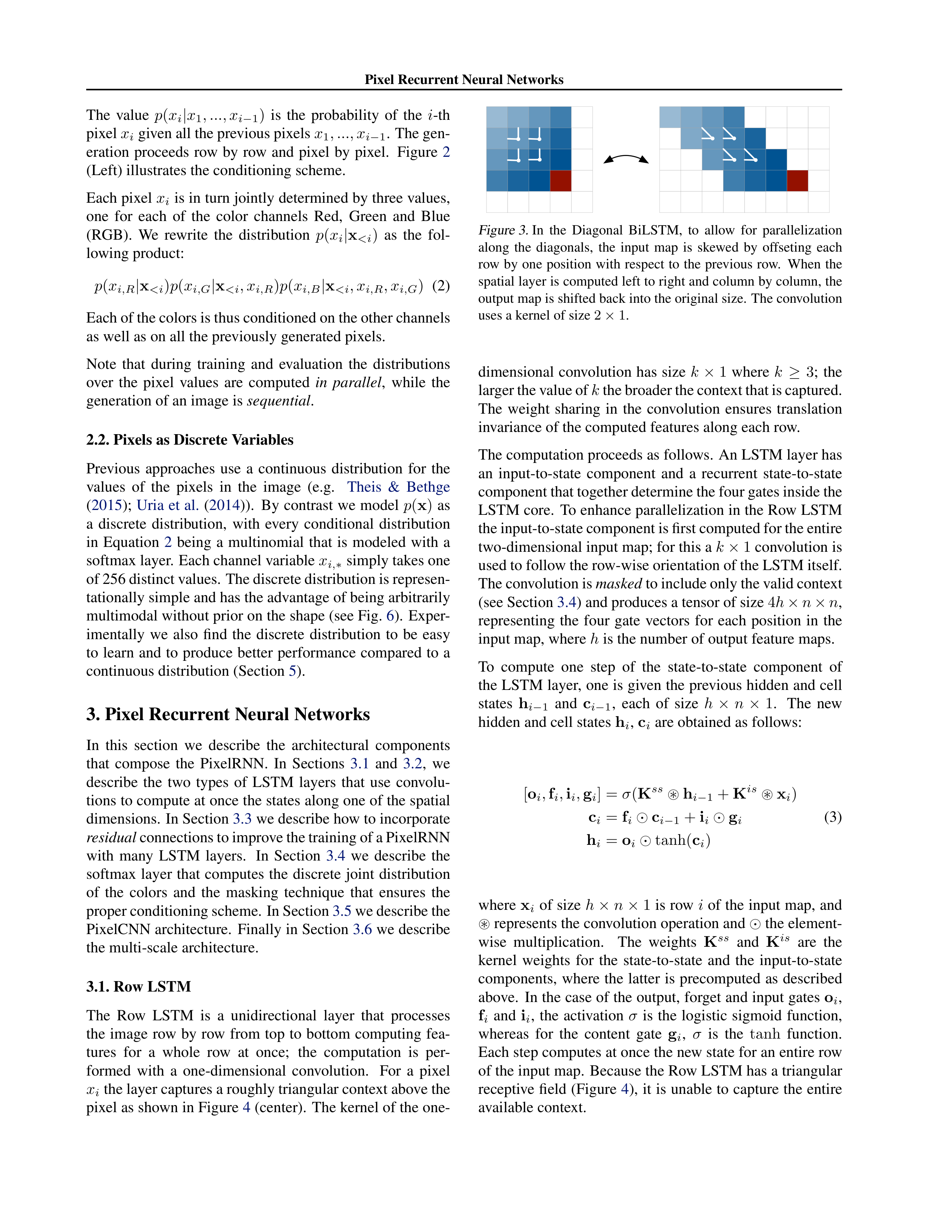
Figure 3.
In
the
Diagonal
BiLSTM,
to
allow
for
parallelization
along
the
diagonals,
the
input
map
is
skewed
by
offseting
each
row
by
one
position
with
respect
to
the
previous
row.
When
the
spatial layer is computed left to right and column by column, the
output map is shifted back into the original size.
The convolution
uses a kernel of size
2
×
1
.
dimensional convolution
has size
k
×
1
where
k
≥
3
;
the
larger the value of
k
the broader the context that is captured.
The
weight
sharing
in
the
convolution
ensures
translation
invariance of the computed features along each row.
The computation proceeds as follows.
An LSTM layer has
an
input-to-state
component
and
a
recurrent
state-to-state
component that together determine the four gates inside the
LSTM core.
To enhance parallelization in the Row LSTM
the input-to-state component is first computed for the entire
two-dimensional input map; for this a
k
×
1
convolution is
used to follow the row-wise orientation of the LSTM itself.
The convolution is
masked
to include only the valid context
(see Section
3.4
) and produces a tensor of size
4
h
×
n
×
n
,
representing
the
four
gate
vectors
for
each
position
in
the
input map, where
h
is the number of output feature maps.
To
compute
one
step
of
the
state-to-state
component
of
the LSTM layer, one is given the previous hidden and cell
states
h
i
−
1
and
c
i
−
1
,
each
of
size
h
×
n
×
1
.
The
new
hidden and cell states
h
i
,
c
i
are obtained as follows:
[
o
i
,
f
i
,
i
i
,
g
i
] =
σ
(
K
ss
⊛
h
i
−
1
+
K
is
⊛
x
i
)
c
i
=
f
i
⊙
c
i
−
1
+
i
i
⊙
g
i
h
i
=
o
i
⊙
tanh(
c
i
)
(3)
where
x
i
of size
h
×
n
×
1
is row
i
of the input map, and
⊛
represents the convolution operation and
⊙
the element-
wise
multiplication.
The
weights
K
ss
and
K
is
are
the
kernel
weights
for
the
state-to-state
and
the
input-to-state
components,
where
the
latter
is
precomputed
as
described
above.
In the case of the output, forget and input gates
o
i
,
f
i
and
i
i
,
the
activation
σ
is
the
logistic
sigmoid
function,
whereas
for
the
content
gate
g
i
,
σ
is
the
tanh
function.
Each step computes at once the new state for an entire row
of the input map.
Because the Row LSTM has a triangular
receptive field (Figure
4
),
it is unable to capture the entire
available context.
Pixel Recurrent Neural Networks
PixelCNN
Row LSTM
Diagonal BiLSTM
Figure 4.
Visualization
of
the
input-to-state
and
state-to-state
mappings for the three proposed architectures.
3.2. Diagonal BiLSTM
The
Diagonal
BiLSTM
is
designed
to
both
parallelize
the
computation and to capture the entire available context for
any
image
size.
Each
of
the
two
directions
of
the
layer
scans
the
image
in
a
diagonal
fashion
starting
from
a
cor-
ner
at
the
top
and
reaching
the
opposite
corner
at
the
bot-
tom.
Each
step
in
the
computation
computes
at
once
the
LSTM state along a diagonal in the image.
Figure
4
(right)
illustrates the computation and the resulting receptive field.
The
diagonal
computation
proceeds
as
follows.
We
first
skew
the
input
map
into
a
space
that
makes
it
easy
to
ap-
ply
convolutions
along
diagonals.
The
skewing
operation
offsets each row of the input map by one position with re-
spect
to
the
previous
row,
as
illustrated
in
Figure
3
;
this
results in a map of size
n
×
(2
n
−
1)
.
At this point we can
compute the input-to-state and state-to-state components of
the Diagonal BiLSTM. For each of the two directions, the
input-to-state component is simply a
1
×
1
convolution
K
is
that contributes to the four gates in the LSTM core; the op-
eration
generates
a
4
h
×
n
×
n
tensor.
The
state-to-state
recurrent component is then computed with a
column-wise
convolution
K
ss
that
has
a
kernel
of
size
2
×
1
.
The
step
takes the previous hidden and cell states, combines the con-
tribution of the input-to-state component and produces the
next
hidden
and
cell
states,
as
defined
in
Equation
3
.
The
output feature map is then skewed back into an
n
×
n
map
by
removing
the
offset
positions.
This
computation
is
re-
peated
for
each
of
the
two
directions.
Given
the
two
out-
put
maps,
to
prevent
the
layer
from
seeing
future
pixels,
the
right
output map
is
then
shifted down
by
one row and
added to the
left
output map.
Besides
reaching
the
full
dependency
field,
the
Diagonal
BiLSTM
has
the
additional
advantage
that
it
uses
a
con-
volutional
kernel
of
size
2
×
1
that
processes
a
minimal
amount of information at each step yielding a highly non-
linear computation.
Kernel sizes larger than
2
×
1
are not
particularly useful as they do not broaden the already global
receptive field of the Diagonal BiLSTM.
3.3. Residual Connections
We
train
PixelRNNs
of
up
to
twelve
layers
of
depth.
As
a means to both increase convergence speed and propagate
signals more directly through the network, we deploy
resid-
ual connections
(
He et al.
,
2015
) from one LSTM layer to
the next.
Figure
5
shows a diagram of the residual blocks.
The
input
map
to
the
PixelRNN
LSTM
layer
has
2
h
fea-
tures.
The input-to-state component reduces the number of
features
by
producing
h
features
per
gate.
After
applying
the recurrent layer, the output map is upsampled back to
2
h
features per position via a
1
×
1
convolution and the input
map is added to the output map.
This method is related to
previous approaches that use gating along the depth of the
recurrent network (
Kalchbrenner et al.
,
2015
;
Zhang et al.
,
2016
),
but
has
the
advantage
of
not
requiring
additional
gates.
Apart
from
residual
connections,
one
can
also
use
learnable
skip
connections
from
each
layer
to
the
output.
In the experiments we evaluate the relative effectiveness of
residual and layer-to-output skip connections.
ReLU - 1x1 Conv
+
ReLU - 3x3 Conv
h
2
h
ReLU - 1x1 Conv
h
2
h
LSTM
+
2
h
1x1 Conv
h
2
h
Figure 5.
Residual blocks for a PixelCNN (left) and PixelRNNs.
3.4. Masked Convolution
The
h
features for each input position at every layer in the
network
are
split
into
three
parts,
each
corresponding
to
one
of
the
RGB
channels.
When
predicting
the
R
chan-
nel
for
the
current
pixel
x
i
,
only
the
generated
pixels
left
and
above
of
x
i
can
be
used
as
context.
When
predicting
the G channel, the value of the R channel can also be used
as
context
in
addition
to
the
previously
generated
pixels.
Likewise,
for
the
B
channel,
the
values
of
both
the
R
and
G channels can be used.
To restrict connections in the net-
work to these dependencies, we apply a
mask
to the input-
to-state convolutions and to other purely convolutional lay-
ers in a PixelRNN.
We
use
two
types
of
masks
that
we
indicate
with
mask
A
and
mask
B
,
as
shown
in
Figure
2
(Right).
Mask
A
is
ap-
plied
only
to
the
first
convolutional
layer
in
a
PixelRNN
and
restricts
the
connections
to
those
neighboring
pixels
and
to
those
colors
in
the
current
pixels
that
have
already
been
predicted.
On
the
other
hand,
mask
B
is
applied
to
all
the
subsequent
input-to-state
convolutional
transitions
and relaxes the restrictions of mask A by also allowing the
connection
from
a
color
to
itself.
The
masks
can
be
eas-
ily implemented by zeroing out the corresponding weights
in the input-to-state convolutions after each update.
Simi-
Pixel Recurrent Neural Networks
PixelCNN
Row LSTM
Diagonal BiLSTM
7
×
7
conv mask A
Multiple residual blocks:
(see fig
5
)
Conv
Row LSTM
Diagonal BiLSTM
3
×
3
mask B
i-s:
3
×
1
mask B
i-s:
1
×
1
mask B
s-s:
3
×
1
no mask
s-s:
1
×
2
no mask
ReLU followed by
1
×
1
conv, mask B (2 layers)
256-way Softmax for each RGB color (Natural images)
or Sigmoid (MNIST)
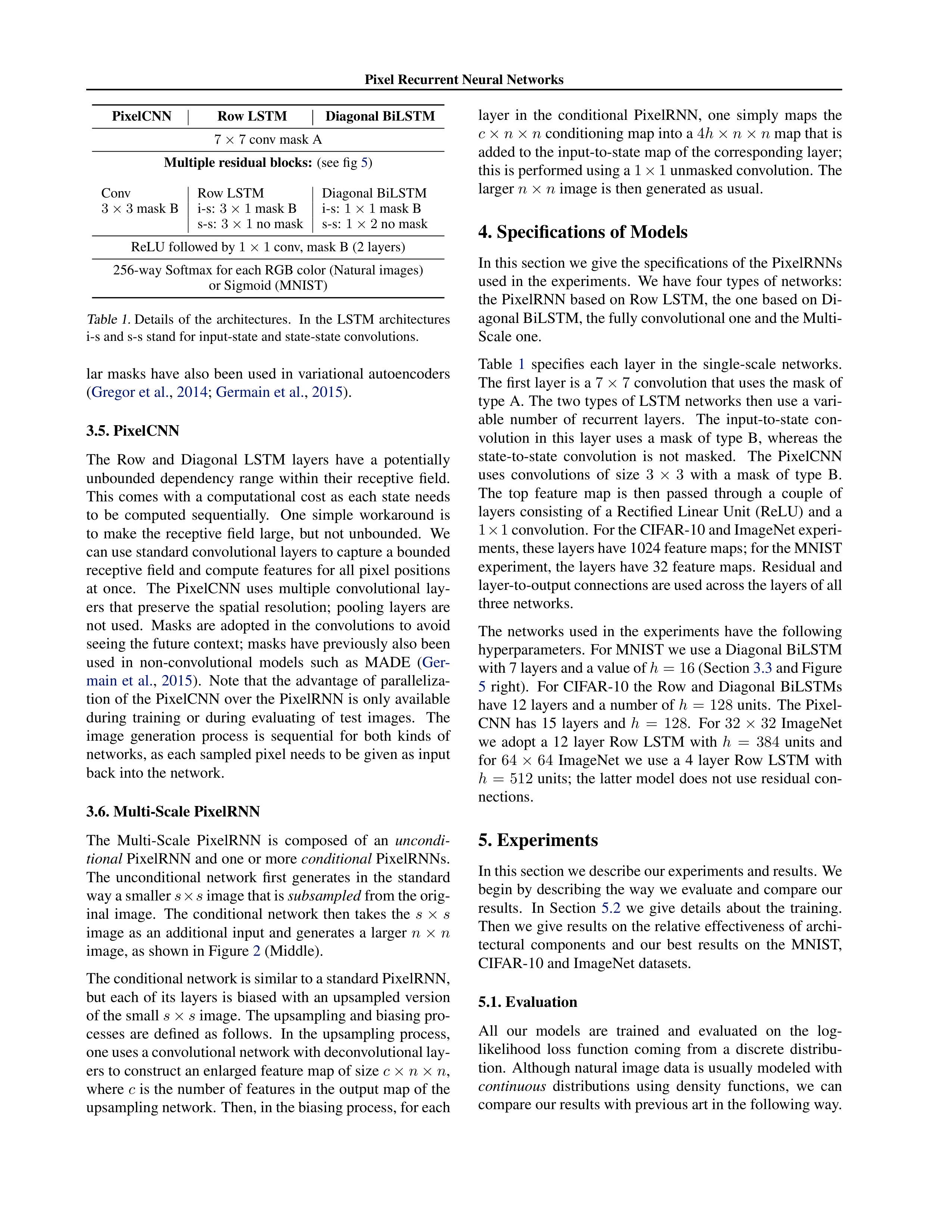
Table 1.
Details
of
the
architectures.
In
the
LSTM
architectures
i-s and s-s stand for input-state and state-state convolutions.
lar
masks
have
also
been
used
in
variational
autoencoders
(
Gregor et al.
,
2014
;
Germain et al.
,
2015
).
3.5. PixelCNN
The
Row
and
Diagonal
LSTM
layers
have
a
potentially
unbounded
dependency
range
within
their
receptive
field.
This
comes
with
a
computational
cost
as
each
state
needs
to
be
computed
sequentially.
One
simple
workaround
is
to
make
the
receptive
field
large,
but
not
unbounded.
We
can use standard convolutional layers to capture a bounded
receptive field and compute features for all pixel positions
at
once.
The
PixelCNN
uses
multiple
convolutional
lay-
ers
that
preserve
the
spatial
resolution;
pooling
layers
are
not
used.
Masks
are
adopted
in
the
convolutions
to
avoid
seeing the future context; masks have previously also been
used
in
non-convolutional
models
such
as
MADE
(
Ger-
main
et
al.
,
2015
).
Note
that
the
advantage
of
paralleliza-
tion of the PixelCNN over the PixelRNN is only available
during
training
or
during
evaluating
of
test
images.
The
image
generation
process
is
sequential
for
both
kinds
of
networks, as each sampled pixel needs to be given as input
back into the network.
3.6. Multi-Scale PixelRNN
The
Multi-Scale
PixelRNN
is
composed
of
an
uncondi-
tional
PixelRNN and one or more
conditional
PixelRNNs.
The
unconditional
network
first
generates
in
the
standard
way a smaller
s
×
s
image that is
subsampled
from the orig-
inal
image.
The
conditional
network
then
takes
the
s
×
s
image
as
an
additional
input
and
generates
a
larger
n
×
n
image, as shown in Figure
2
(Middle).
The conditional network is similar to a standard PixelRNN,
but
each
of
its
layers
is
biased
with
an
upsampled
version
of the small
s
×
s
image.
The upsampling and biasing pro-
cesses
are
defined
as
follows.
In
the
upsampling
process,
one uses a convolutional network with deconvolutional lay-
ers to construct an enlarged feature map of size
c
×
n
×
n
,
where
c
is the number of features in the output map of the
upsampling network.
Then, in the biasing process, for each
layer
in
the
conditional
PixelRNN,
one
simply
maps
the
c
×
n
×
n
conditioning map into a
4
h
×
n
×
n
map that is
added to the input-to-state map of the corresponding layer;
this is performed using a
1
×
1
unmasked convolution.
The
larger
n
×
n
image is then generated as usual.
4. Specifications of Models
In this section we give the specifications of the PixelRNNs
used in the experiments.
We have four types of networks:
the PixelRNN based on Row LSTM, the one based on Di-
agonal BiLSTM, the fully convolutional one and the Multi-
Scale one.
Table
1
specifies
each
layer
in
the
single-scale
networks.
The first layer is a
7
×
7
convolution that uses the mask of
type A. The two types of LSTM networks then use a vari-
able
number
of
recurrent
layers.
The
input-to-state
con-
volution
in
this
layer
uses
a
mask
of
type
B,
whereas
the
state-to-state
convolution
is
not
masked.
The
PixelCNN
uses
convolutions
of
size
3
×
3
with
a
mask
of
type
B.
The
top
feature
map
is
then
passed
through
a
couple
of
layers
consisting
of
a
Rectified
Linear
Unit
(ReLU)
and
a
1
×
1
convolution. For the CIFAR-10 and ImageNet experi-
ments, these layers have 1024 feature maps; for the MNIST
experiment, the layers have 32 feature maps.
Residual and
layer-to-output connections are used across the layers of all
three networks.
The
networks
used
in
the
experiments
have
the
following
hyperparameters.
For MNIST we use a Diagonal BiLSTM
with 7 layers and a value of
h
= 16
(Section
3.3
and Figure
5
right).
For
CIFAR-10
the
Row
and
Diagonal
BiLSTMs
have 12 layers and a number of
h
=
128
units.
The Pixel-
CNN
has
15
layers
and
h
=
128
.
For
32
×
32
ImageNet
we
adopt
a
12
layer
Row
LSTM
with
h
=
384
units
and
for
64
×
64
ImageNet
we
use
a
4
layer
Row
LSTM
with
h
=
512
units; the latter model does not use residual con-
nections.
5. Experiments
In this section we describe our experiments and results. We
begin by describing the way we evaluate and compare our
results.
In
Section
5.2
we
give
details
about
the
training.
Then we give results on the relative effectiveness of archi-
tectural
components
and
our
best
results
on
the
MNIST,
CIFAR-10 and ImageNet datasets.
5.1. Evaluation
All
our
models
are
trained
and
evaluated
on
the
log-
likelihood
loss
function
coming
from
a
discrete
distribu-
tion.
Although natural image data is usually modeled with
continuous
distributions
using
density
functions,
we
can
compare our results with previous art in the following way.
Pixel Recurrent Neural Networks
In
the
literature
it
is
currently
best
practice
to
add
real-
valued noise to the pixel values to dequantize the data when
using density functions (
Uria et al.
,
2013
).
When uniform
noise is added (with values in the interval [0, 1]),
then the
log-likelihoods
of
continuous
and
discrete
models
are
di-
rectly comparable (
Theis et al.
,
2015
).
In our case, we can
use the values from the discrete distribution as a piecewise-
uniform
continuous
function
that
has
a
constant
value
for
every interval
[
i, i
+ 1]
, i
=
1
,
2
, . . .
256
.
This correspond-
ing distribution will have the same log-likelihood (on data
with
added
noise)
as
the
original
discrete
distribution
(on
discrete data).
For
MNIST
we
report
the
negative
log-likelihood
in
nats
as
it
is
common
practice
in
literature.
For
CIFAR-10
and
ImageNet we report negative log-likelihoods in
bits
per di-
mension. The total discrete log-likelihood is normalized by
the dimensionality of the images (e.g.,
32
×
32
×
3 = 3072
for
CIFAR-10).
These
numbers
are
interpretable
as
the
number
of
bits
that
a
compression
scheme
based
on
this
model
would
need
to
compress
every
RGB
color
value
(
van den Oord & Schrauwen
,
2014b
;
Theis et al.
,
2015
);
in practice there is also a small overhead due to arithmetic
coding.
5.2. Training Details
Our models are trained on GPUs using the Torch toolbox.
From the different parameter update rules tried, RMSProp
gives best convergence performance and is used for all ex-
periments.
The
learning
rate
schedules
were
manually
set
for every dataset to the highest values that allowed fast con-
vergence.
The
batch
sizes
also
vary
for
different
datasets.
For smaller datasets such as MNIST and CIFAR-10 we use
smaller batch sizes of 16 images as this seems to regularize
the
models.
For
ImageNet
we
use
as
large
a
batch
size
as
allowed
by
the
GPU
memory;
this
corresponds
to
64
im-
ages/batch for
32
×
32
ImageNet, and 32 images/batch for
64
×
64
ImageNet.
Apart
from
scaling
and
centering
the
images at the input of the network, we don’t use any other
preprocessing
or
augmentation.
For
the
multinomial
loss
function
we
use
the
raw
pixel
color
values
as
categories.
For all the PixelRNN models, we learn the initial recurrent
state of the network.
5.3. Discrete Softmax Distribution
Apart from being intuitive and easy to implement, we find
that
using
a
softmax
on
discrete
pixel
values
instead
of
a
mixture density approach on continuous pixel values gives
better
results.
For
the
Row
LSTM
model
with
a
softmax
output distribution we obtain 3.06 bits/dim on the CIFAR-
10
validation
set.
For
the
same
model
with
a
Mixture
of
Conditional Gaussian Scale Mixtures (MCGSM) (
Theis &
Bethge
,
2015
) we obtain 3.22 bits/dim.
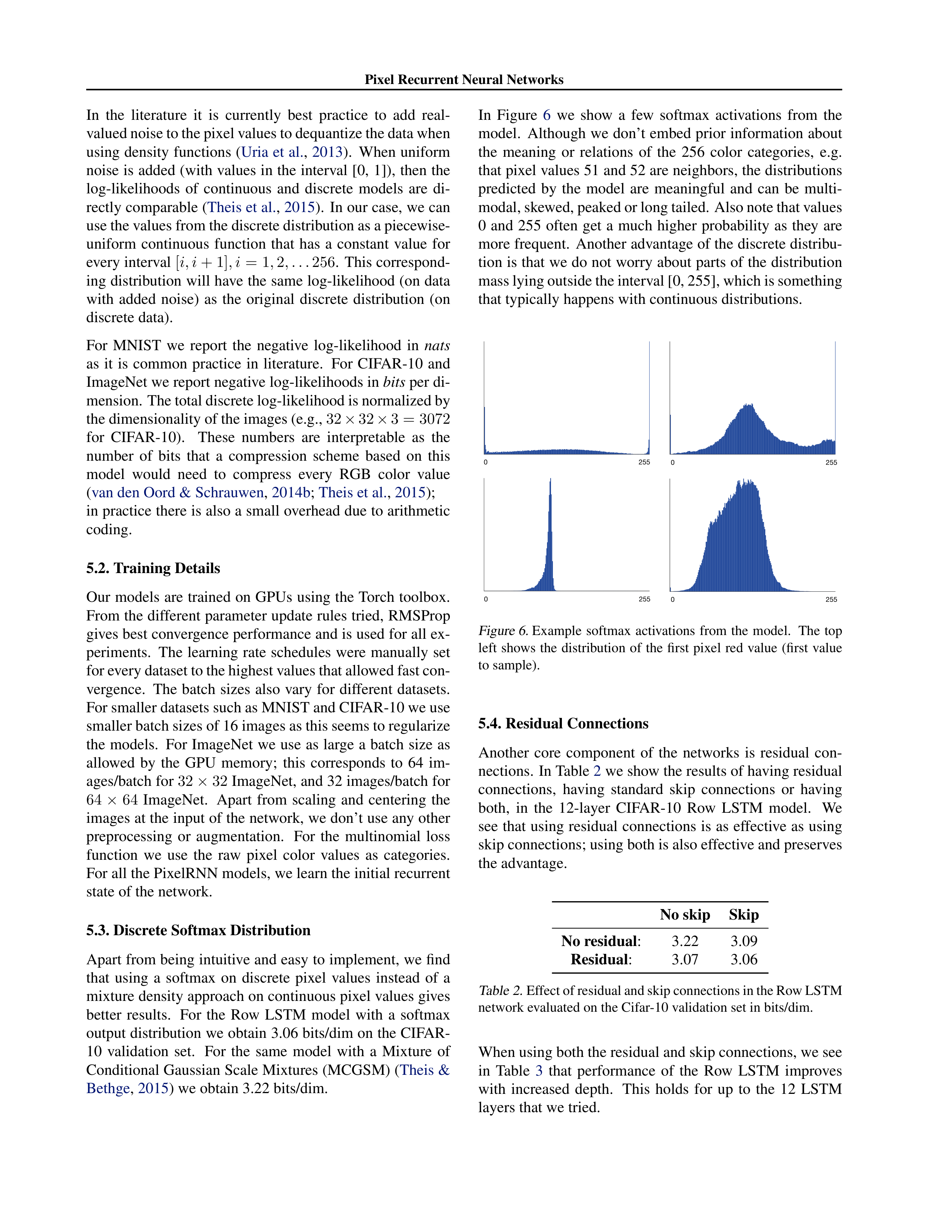
In
Figure
6
we
show
a
few
softmax
activations
from
the
model.
Although we don’t embed prior information about
the
meaning
or
relations
of
the
256
color
categories,
e.g.
that pixel values 51 and 52 are neighbors, the distributions
predicted
by
the
model
are
meaningful
and
can
be
multi-
modal, skewed, peaked or long tailed. Also note that values
0
and
255
often
get
a
much
higher
probability
as
they
are
more frequent.
Another advantage of the discrete distribu-
tion is that we do not worry about parts of the distribution
mass lying outside the interval [0, 255], which is something
that typically happens with continuous distributions.
0
50
100
150
200
250
0
50
100
150
200
250
0
50
100
150
200
250
0
50
100
150
200
250
0 255
0 255
0 255
0 255
0 255
Figure 6.
Example
softmax
activations
from
the
model.
The
top
left
shows
the
distribution
of
the
first
pixel
red
value
(first
value
to sample).
5.4. Residual Connections
Another
core
component
of
the
networks
is
residual
con-
nections.
In Table
2
we show the results of having residual
connections,
having
standard
skip
connections
or
having
both,
in
the
12-layer
CIFAR-10
Row
LSTM
model.
We
see that using residual connections is as effective as using
skip connections; using both is also effective and preserves
the advantage.
No skip
Skip
No residual
:
3.22
3.09
Residual
:
3.07
3.06
Table 2.
Effect of residual and skip connections in the Row LSTM
network evaluated on the Cifar-10 validation set in bits/dim.
When using both the residual and skip connections, we see
in
Table
3
that
performance
of
the
Row
LSTM
improves
with
increased
depth.
This
holds
for
up
to
the
12
LSTM
layers that we tried.
Pixel Recurrent Neural Networks
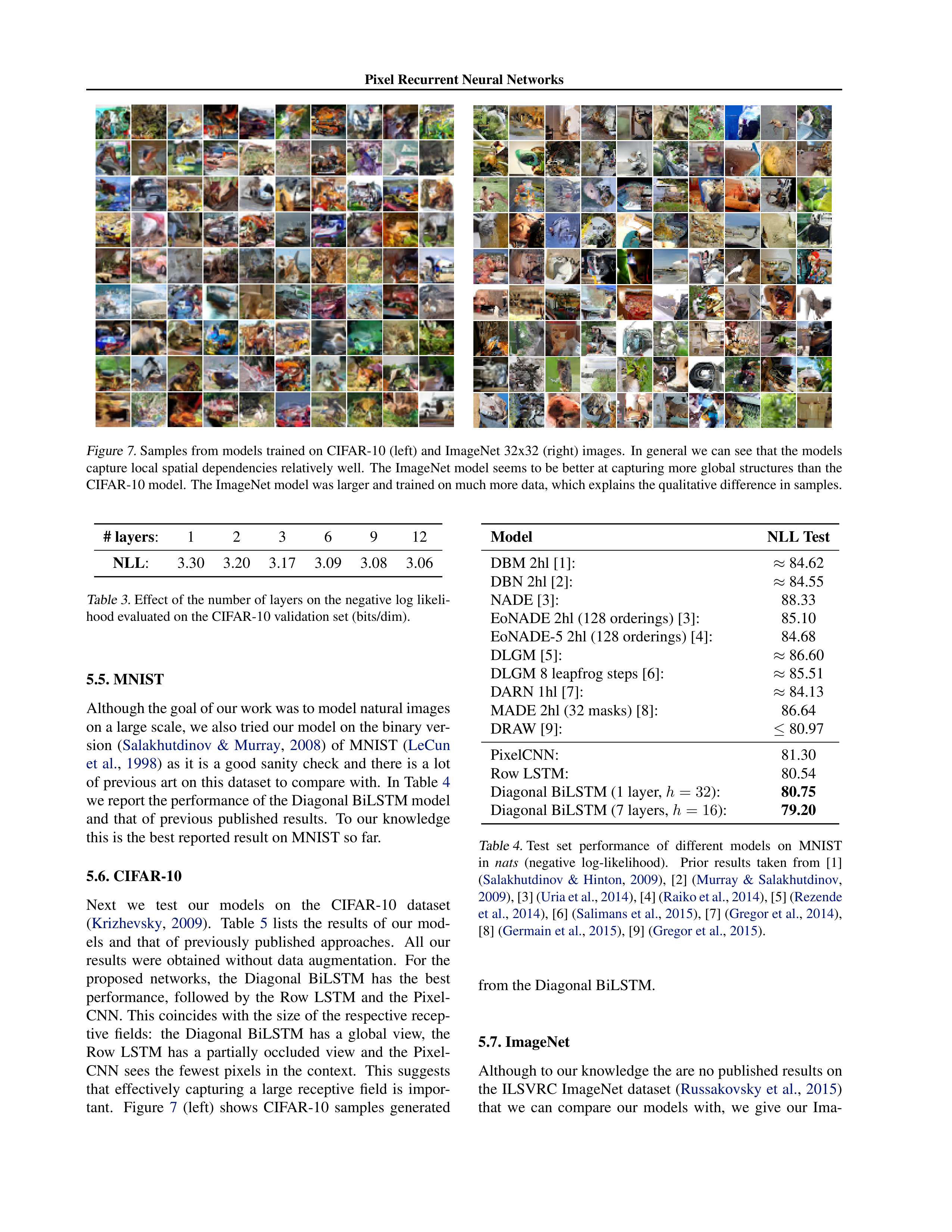
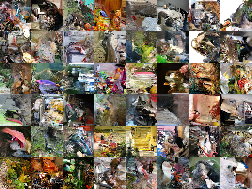
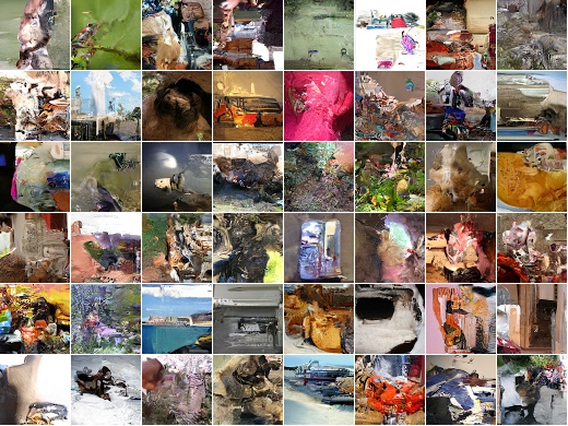
Figure 7.
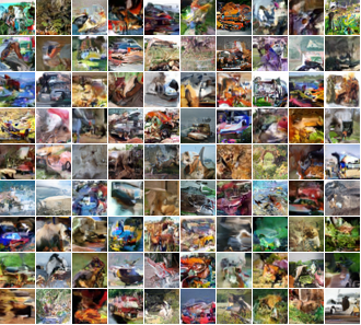
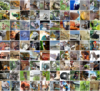
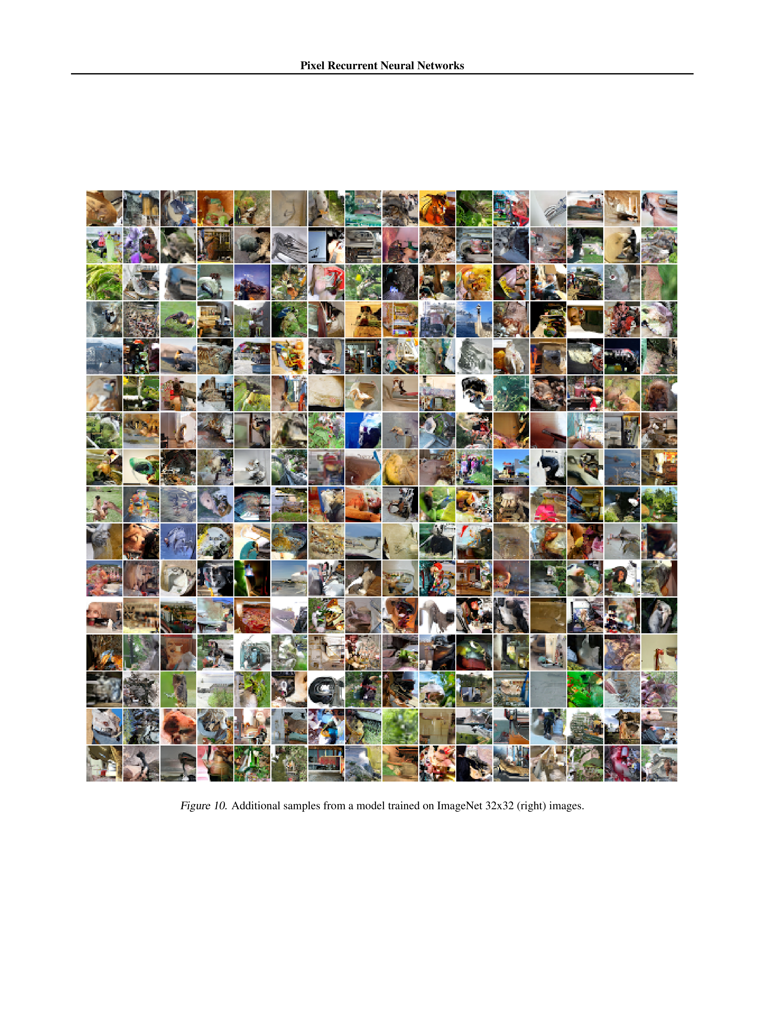
Samples from models trained on CIFAR-10 (left) and ImageNet 32x32 (right) images.
In general we can see that the models
capture local spatial dependencies relatively well.
The ImageNet model seems to be better at capturing more global structures than the
CIFAR-10 model.
The ImageNet model was larger and trained on much more data, which explains the qualitative difference in samples.
# layers
:
1
2
3
6
9
12
NLL
:
3.30
3.20
3.17
3.09
3.08
3.06
Table 3.
Effect of the number of layers on the negative log likeli-
hood evaluated on the CIFAR-10 validation set (bits/dim).
5.5. MNIST
Although the goal of our work was to model natural images
on a large scale, we also tried our model on the binary ver-
sion
(
Salakhutdinov
&
Murray
,
2008
)
of
MNIST
(
LeCun
et
al.
,
1998
)
as
it
is
a
good
sanity
check
and
there
is
a
lot
of previous art on this dataset to compare with.
In Table
4
we report the performance of the Diagonal BiLSTM model
and
that
of
previous
published
results.
To
our
knowledge
this is the best reported result on MNIST so far.
5.6. CIFAR-10
Next
we
test
our
models
on
the
CIFAR-10
dataset
(
Krizhevsky
,
2009
).
Table
5
lists
the
results
of
our
mod-
els
and
that
of
previously
published
approaches.
All
our
results
were
obtained
without
data
augmentation.
For
the
proposed
networks,
the
Diagonal
BiLSTM
has
the
best
performance,
followed
by
the
Row
LSTM
and
the
Pixel-
CNN. This coincides with the size of the respective recep-
tive
fields:
the
Diagonal
BiLSTM
has
a
global
view,
the
Row
LSTM
has
a
partially
occluded
view
and
the
Pixel-
CNN
sees
the
fewest
pixels
in
the
context.
This
suggests
that
effectively
capturing
a
large
receptive
field
is
impor-
tant.
Figure
7
(left)
shows
CIFAR-10
samples
generated
Model
NLL Test
DBM 2hl [1]:
≈
84.62
DBN 2hl [2]:
≈
84.55
NADE [3]:
88.33
EoNADE 2hl (128 orderings) [3]:
85.10
EoNADE-5 2hl (128 orderings) [4]:
84.68
DLGM [5]:
≈
86.60
DLGM 8 leapfrog steps [6]:
≈
85.51
DARN 1hl [7]:
≈
84.13
MADE 2hl (32 masks) [8]:
86.64
DRAW [9]:
≤
80.97
PixelCNN:
81.30
Row LSTM:
80.54
Diagonal BiLSTM (1 layer,
h
= 32
):
80.75
Diagonal BiLSTM (7 layers,
h
= 16
):
79.20
Table 4.
Test
set
performance
of
different
models
on
MNIST
in
nats
(negative
log-likelihood).
Prior
results
taken
from
[1]
(
Salakhutdinov
&
Hinton
,
2009
),
[2]
(
Murray
&
Salakhutdinov
,
2009
), [3] (
Uria et al.
,
2014
), [4] (
Raiko et al.
,
2014
), [5] (
Rezende
et al.
,
2014
), [6] (
Salimans et al.
,
2015
), [7] (
Gregor et al.
,
2014
),
[8] (
Germain et al.
,
2015
), [9] (
Gregor et al.
,
2015
).
from the Diagonal BiLSTM.
5.7. ImageNet
Although to our knowledge the are no published results on
the
ILSVRC
ImageNet
dataset
(
Russakovsky
et
al.
,
2015
)
that
we
can
compare
our
models
with,
we
give
our
Ima-
Pixel Recurrent Neural Networks
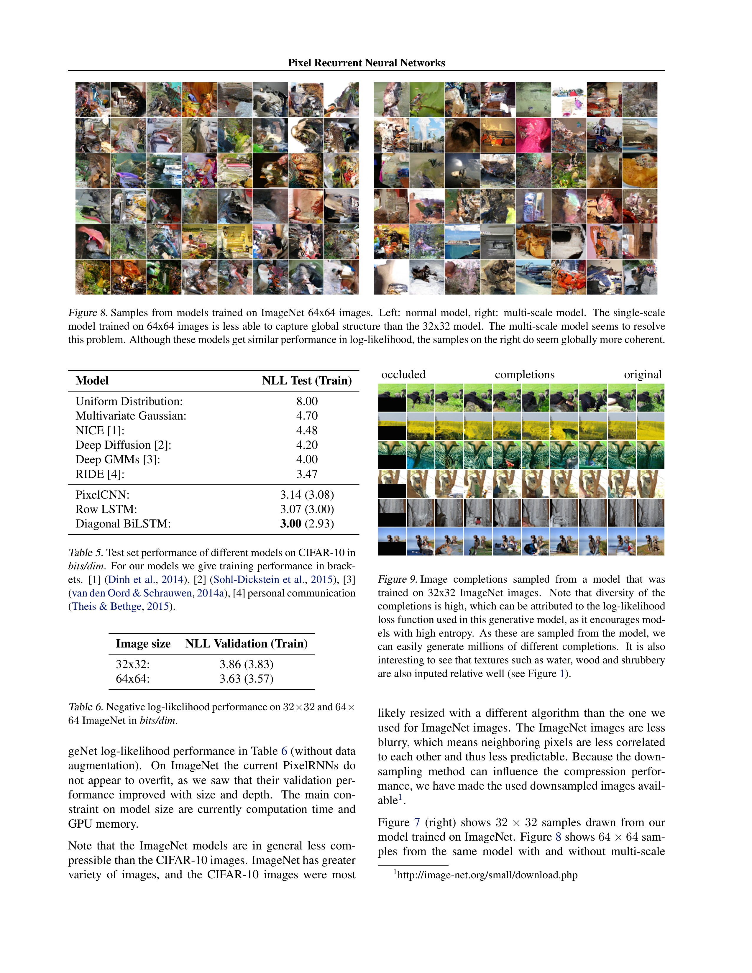
Figure 8.
Samples
from
models
trained
on
ImageNet
64x64
images.
Left:
normal
model,
right:
multi-scale
model.
The
single-scale
model trained on 64x64 images is less able to capture global structure than the 32x32 model.
The multi-scale model seems to resolve
this problem. Although these models get similar performance in log-likelihood, the samples on the right do seem globally more coherent.
Model
NLL Test (Train)
Uniform Distribution:
8.00
Multivariate Gaussian:
4.70
NICE [1]:
4.48
Deep Diffusion [2]:
4.20
Deep GMMs [3]:
4.00
RIDE [4]:
3.47
PixelCNN:
3.14 (3.08)
Row LSTM:
3.07 (3.00)
Diagonal BiLSTM:
3.00
(2.93)
Table 5.
Test set performance of different models on CIFAR-10 in
bits/dim
.
For our models we give training performance in brack-
ets.
[1]
(
Dinh
et
al.
,
2014
),
[2]
(
Sohl-Dickstein
et
al.
,
2015
),
[3]
(
van den Oord & Schrauwen
,
2014a
), [4] personal communication
(
Theis & Bethge
,
2015
).
Image size
NLL Validation (Train)
32x32:
3.86 (3.83)
64x64:
3.63 (3.57)
Table 6.
Negative log-likelihood performance on
32
×
32
and
64
×
64
ImageNet in
bits/dim
.
geNet log-likelihood performance in Table
6
(without data
augmentation).
On
ImageNet
the
current
PixelRNNs
do
not
appear
to
overfit,
as
we
saw
that
their
validation
per-
formance
improved
with
size
and
depth.
The
main
con-
straint
on
model
size
are
currently
computation
time
and
GPU memory.
Note
that
the
ImageNet
models
are
in
general
less
com-
pressible than the CIFAR-10 images.
ImageNet has greater
variety
of
images,
and
the
CIFAR-10
images
were
most
occluded
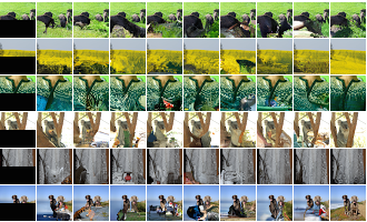
completions
original
Figure 9.
Image
completions
sampled
from
a
model
that
was
trained
on
32x32
ImageNet
images.
Note
that
diversity
of
the
completions is high, which can be attributed to the log-likelihood
loss function used in this generative model, as it encourages mod-
els with high entropy.
As these are sampled from the model,
we
can
easily
generate
millions
of
different
completions.
It
is
also
interesting to see that textures such as water, wood and shrubbery
are also inputed relative well (see Figure
1
).
likely
resized
with
a
different
algorithm
than
the
one
we
used for ImageNet images.
The ImageNet images are less
blurry, which means neighboring pixels are less correlated
to each other and thus less predictable.
Because the down-
sampling
method
can
influence
the
compression
perfor-
mance, we have made the used downsampled images avail-
able
1
.
Figure
7
(right)
shows
32
×
32
samples
drawn
from
our
model trained on ImageNet.
Figure
8
shows
64
×
64
sam-
ples
from
the
same
model
with
and
without
multi-scale
1
http://image-net.org/small/download.php
Pixel Recurrent Neural Networks
conditioning.
Finally,
we
also
show
image
completions
sampled from the model in Figure
9
.
6. Conclusion
In this paper we significantly improve and build upon deep
recurrent neural networks as generative models for natural
images.
We have described novel two-dimensional LSTM
layers:
the
Row
LSTM
and
the
Diagonal
BiLSTM,
that
scale
more
easily
to
larger
datasets.
The
models
were
trained to model the raw RGB pixel values.
We treated the
pixel
values
as
discrete
random
variables
by
using
a
soft-
max
layer
in
the
conditional
distributions.
We
employed
masked convolutions to allow PixelRNNs to model full de-
pendencies
between
the
color
channels.
We
proposed
and
evaluated
architectural
improvements
in
these
models
re-
sulting in PixelRNNs with up to 12 LSTM layers.
We
have
shown
that
the
PixelRNNs
significantly
improve
the state of the art on the MNIST and CIFAR-10 datasets.
We
also
provide
new
benchmarks
for
generative
image
modeling
on
the
ImageNet
dataset.
Based
on
the
samples
and
completions
drawn
from
the
models
we
can
conclude
that
the
PixelRNNs
are
able
to
model
both
spatially
local
and long-range correlations and are able to produce images
that
are
sharp
and
coherent.
Given
that
these
models
im-
prove as we make them larger and that there is practically
unlimited data available to train on, more computation and
larger models are likely to further improve the results.
Acknowledgements
The authors would like to thank Shakir Mohamed and Guil-
laume
Desjardins
for
helpful
input
on
this
paper
and
Lu-
cas Theis, Alex Graves, Karen Simonyan, Lasse Espeholt,
Danilo
Rezende,
Karol
Gregor
and
Ivo
Danihelka
for
in-
sightful discussions.
References
Bengio,
Yoshua
and
Bengio,
Samy.
Modeling
high-
dimensional
discrete
data
with
multi-layer
neural
net-
works.
pp. 400–406. MIT Press, 2000.
Dinh,
Laurent,
Krueger,
David,
and
Bengio,
Yoshua.
NICE:
Non-linear
independent
components
estimation.
arXiv preprint arXiv:1410.8516
, 2014.
Germain,
Mathieu,
Gregor,
Karol,
Murray,
Iain,
and
Larochelle, Hugo.
MADE: Masked autoencoder for dis-
tribution
estimation.
arXiv
preprint
arXiv:1502.03509
,
2015.
Graves, Alex.
Generating sequences with recurrent neural
networks.
arXiv preprint arXiv:1308.0850
, 2013.
Graves, Alex and Schmidhuber, J¨urgen.
Offline handwrit-
ing
recognition
with
multidimensional
recurrent
neural
networks.
In
Advances
in
Neural
Information
Process-
ing Systems
, 2009.
Gregor,
Karol,
Danihelka,
Ivo,
Mnih,
Andriy,
Blundell,
Charles,
and
Wierstra,
Daan.
Deep
autoregressive
net-
works.
In
Proceedings of the 31st International Confer-
ence on Machine Learning
, 2014.
Gregor, Karol, Danihelka, Ivo, Graves, Alex, and Wierstra,
Daan.
DRAW:
A
recurrent
neural
network
for
image
generation.
Proceedings of the 32nd International Con-
ference on Machine Learning
, 2015.
He,
Kaiming,
Zhang,
Xiangyu,
Ren,
Shaoqing,
and
Sun,
Jian. Deep residual learning for image recognition.
arXiv
preprint arXiv:1512.03385
, 2015.
Hochreiter,
Sepp
and
Schmidhuber,
J¨urgen.
Long
short-
term memory.
Neural computation
, 1997.
Kalchbrenner, Nal and Blunsom, Phil.
Recurrent continu-
ous translation models.
In
Proceedings of the 2013 Con-
ference on Empirical Methods in Natural Language Pro-
cessing
, 2013.
Kalchbrenner,
Nal,
Danihelka,
Ivo,
and
Graves,
Alex.
Grid
long
short-term
memory.
arXiv
preprint
arXiv:1507.01526
, 2015.
Kingma,
Diederik
P
and
Welling,
Max.
Auto-encoding
variational
bayes.
arXiv
preprint
arXiv:1312.6114
,
2013.
Krizhevsky,
Alex.
Learning
multiple
layers
of
features
from tiny images.
2009.
Larochelle,
Hugo
and
Murray,
Iain.
The
neural
autore-
gressive distribution estimator.
The Journal of Machine
Learning Research
, 2011.
LeCun, Yann, Bottou, L´eon, Bengio, Yoshua, and Haffner,
Patrick.
Gradient-based
learning
applied
to
document
recognition.
Proceedings of the IEEE
, 1998.
Murray,
Iain
and
Salakhutdinov,
Ruslan
R.
Evaluat-
ing
probabilities
under
high-dimensional
latent
variable
models.
In
Advances in Neural Information Processing
Systems
, 2009.
Neal,
Radford
M.
Connectionist
learning
of
belief
net-
works.
Artificial intelligence
, 1992.
Raiko,
Tapani,
Li,
Yao,
Cho,
Kyunghyun,
and
Bengio,
Yoshua.
Iterative
neural
autoregressive
distribution
es-
timator
NADE-k.
In
Advances
in
Neural
Information
Processing Systems
, 2014.
Pixel Recurrent Neural Networks
Rezende, Danilo J, Mohamed, Shakir, and Wierstra, Daan.
Stochastic
backpropagation
and
approximate
inference
in
deep
generative
models.
In
Proceedings
of
the
31st
International Conference on Machine Learning
, 2014.
Russakovsky, Olga, Deng, Jia, Su, Hao, Krause, Jonathan,
Satheesh,
Sanjeev,
Ma,
Sean,
Huang,
Zhiheng,
Karpa-
thy,
Andrej,
Khosla,
Aditya,
Bernstein,
Michael,
Berg,
Alexander
C.,
and
Fei-Fei,
Li.
ImageNet
Large
Scale
Visual Recognition Challenge.
International Journal of
Computer Vision (IJCV)
, 2015.
Salakhutdinov, Ruslan and Hinton, Geoffrey E. Deep boltz-
mann
machines.
In
International
Conference
on
Artifi-
cial Intelligence and Statistics
, 2009.
Salakhutdinov,
Ruslan and Murray,
Iain.
On the quantita-
tive analysis of deep belief networks.
In
Proceedings of
the 25th international conference on Machine learning
,
2008.
Salimans,
Tim,
Kingma,
Diederik
P,
and
Welling,
Max.
Markov
chain
monte
carlo
and
variational
inference:
Bridging the gap.
Proceedings of the 32nd International
Conference on Machine Learning
, 2015.
Sohl-Dickstein, Jascha, Weiss, Eric A., Maheswaranathan,
Niru,
and
Ganguli,
Surya.
Deep
unsupervised
learning
using
nonequilibrium
thermodynamics.
Proceedings
of
the
32nd
International
Conference
on
Machine
Learn-
ing
, 2015.
Stollenga,
Marijn
F,
Byeon,
Wonmin,
Liwicki,
Marcus,
and
Schmidhuber,
Juergen.
Parallel
multi-dimensional
lstm, with application to fast biomedical volumetric im-
age
segmentation.
In
Advances
in
Neural
Information
Processing Systems 28
. 2015.
Sutskever,
Ilya,
Martens,
James,
and
Hinton,
Geoffrey
E.
Generating text with recurrent neural networks.
In
Pro-
ceedings
of
the
28th
International
Conference
on
Ma-
chine Learning
, 2011.
Theis, Lucas and Bethge, Matthias. Generative image mod-
eling using spatial LSTMs.
In
Advances in Neural Infor-
mation Processing Systems
, 2015.
Theis, Lucas, van den Oord, A¨aron, and Bethge, Matthias.
A
note
on
the
evaluation
of
generative
models.
arXiv
preprint arXiv:1511.01844
, 2015.
Uria,
Benigno,
Murray,
Iain,
and
Larochelle,
Hugo.
RNADE: The real-valued neural autoregressive density-
estimator. In
Advances in Neural Information Processing
Systems
, 2013.
Uria,
Benigno,
Murray,
Iain,
and
Larochelle,
Hugo.
A
deep
and
tractable
density
estimator.
In
Proceedings
of
the 31st International Conference on Machine Learning
,
2014.
van den Oord, A¨aron and Schrauwen, Benjamin.
Factoring
variations in natural images with deep gaussian mixture
models.
In
Advances in Neural Information Processing
Systems
, 2014a.
van
den
Oord,
A¨aron
and
Schrauwen,
Benjamin.
The
student-t mixture as a natural image patch prior with ap-
plication to image compression.
The Journal of Machine
Learning Research
, 2014b.
Zhang, Yu, Chen, Guoguo, Yu, Dong, Yao, Kaisheng, Khu-
danpur, Sanjeev, and Glass, James.
Highway long short-
term
memory
RNNs
for
distant
speech
recognition.
In
Proceedings
of
the
International
Conference
on
Acous-
tics, Speech and Signal Processing
, 2016.
Pixel Recurrent Neural Networks
Figure 10.
Additional samples from a model trained on ImageNet 32x32 (right) images.