arXiv:1409.1556v6 [cs.CV] 10 Apr 2015
Published as a conference paper at ICLR 2015
V
ERY
D
EEP
C
ONVOLUTIONAL
N
ETWORKS
FOR
L
ARGE
-S
CALE
I
MAGE
R
ECOGNITION
Karen Simonyan
∗
& Andrew Zisserman
+
Visual Geometry Group, Department of Engineering Science, University of Oxford
{
karen,az
}
@robots.ox.ac.uk
A
BSTRACT
In
this
work
we
investigate
the
effect
of
the
convolutional
network
depth
on
its
accuracy
in
the
large-scale
image
recognition
setting.
Our
main
contribution
is
a thorough evaluation of networks of increasing depth using an architecture with
very small (
3
×
3
) convolution filters, which shows that a significant improvement
on
the
prior-art
configurations
can
be
achieved
by
pushing
the
depth
to
16–19
weight
layers.
These
findings
were
the
basis
of
our
ImageNet
Challenge
2014
submission, where our team secured the first and the second places in the localisa-
tion and classification tracks respectively.
We
also show that our representations
generalise well
to
other datasets,
where
they achieve state-of-the-art results.
We
have made our two best-performing ConvNet models publicly available to facili-
tate further research on the use of deep visual representations in computer vision.
1
I
NTRODUCTION
Convolutional
networks
(ConvNets)
have
recently
enjoyed
a
great
success
in
large-scale
im-
age
and
video
recognition
(Krizhevsky et al.,
2012;
Zeiler & Fergus,
2013;
Sermanet et al.,
2014;
Simonyan & Zisserman,
2014)
which has become possible due to the large public image reposito-
ries, such as ImageNet (Deng et al., 2009), and high-performance computing systems, such as GPUs
or large-scale distributed clusters (Dean et al., 2012).
In particular, an important role in the advance
of deep visual recognition architectures has been played by the ImageNet Large-Scale Visual Recog-
nition
Challenge
(ILSVRC)
(Russakovsky et al.,
2014),
which
has
served
as
a
testbed
for
a
few
generations of large-scale image classification systems, from high-dimensional shallow feature en-
codings (Perronnin et al., 2010) (the winner of ILSVRC-2011) to deep ConvNets (Krizhevsky et al.,
2012) (the winner of ILSVRC-2012).
With
ConvNets
becoming
more
of
a
commodity
in
the
computer
vision
field,
a
number
of
at-
tempts
have
been
made
to
improve
the
original
architecture
of
Krizhevsky et al.
(2012)
in
a
bid
to
achieve
better
accuracy.
For
instance,
the
best-performing
submissions
to
the
ILSVRC-
2013
(Zeiler & Fergus,
2013;
Sermanet et al.,
2014)
utilised
smaller
receptive
window
size
and
smaller
stride
of
the
first
convolutional
layer.
Another
line
of
improvements
dealt
with
training
and
testing
the
networks
densely
over
the
whole
image
and
over
multiple
scales
(Sermanet et al.,
2014;
Howard, 2014).
In this paper, we
address another important aspect
of ConvNet architecture
design – its depth. To this end, we fix other parameters of the architecture, and steadily increase the
depth of the network by adding more convolutional layers, which is feasible due to the use of very
small (
3
×
3
) convolution filters in all layers.
As
a
result,
we
come
up
with
significantly
more
accurate
ConvNet
architectures,
which
not
only
achieve
the
state-of-the-art accuracy on
ILSVRC
classification
and
localisation
tasks,
but
are
also
applicable to other image recognition datasets, where they achieve excellent performance even when
used as a part of a relatively simple pipelines (e.g. deep features classified by a linear SVM without
fine-tuning). We have released our two best-performing models
1
to facilitate further research.
The rest
of the paper is organised as follows.
In Sect. 2,
we
describe our ConvNet configurations.
The details of the image classification training and evaluation are then presented in Sect. 3, and the
∗
current affiliation: Google DeepMind
+
current affiliation:
University of Oxford and Google DeepMind
1
http://www.robots.ox.ac.uk/˜vgg/research/very_deep/
1
Published as a conference paper at ICLR 2015
configurations
are
compared
on
the
ILSVRC
classification
task
in
Sect.
4.
Sect.
5
concludes
the
paper.
For completeness, we also describe and assess our ILSVRC-2014 object localisation system
in Appendix A, and discuss the generalisation of very deep features to other datasets in Appendix B.
Finally, Appendix C contains the list of major paper revisions.
2
C
ONV
N
ET
C
ONFIGURATIONS
To
measure
the
improvement
brought
by
the
increased
ConvNet
depth
in
a
fair
setting,
all
our
ConvNet
layer
configurations
are
designed
using
the
same
principles,
inspired
by
Ciresan et al.
(2011); Krizhevsky et al. (2012).
In this section, we first describe a generic layout of our ConvNet
configurations (Sect. 2.1) and then detail the specific configurations used in the evaluation (Sect. 2.2).
Our design choices are then discussed and compared to the prior art in Sect. 2.3.
2.1
A
RCHITECTURE
During
training,
the
input
to
our
ConvNets
is
a
fixed-size
224
×
224
RGB
image.
The
only
pre-
processing we do is subtracting the mean RGB value, computed on the training set, from each pixel.
The image is passed through a stack of convolutional (conv.) layers, where we use filters with a very
small receptive field:
3
×
3
(which is the smallest size to capture the notion of left/right, up/down,
center).
In one of the configurations we also utilise
1
×
1
convolution filters, which can be seen as
a linear transformation of the input channels (followed by non-linearity).
The convolution stride is
fixed to
1
pixel; the spatial padding of conv. layer input is such that the spatial resolution is preserved
after convolution, i.e. the padding is
1
pixel for
3
×
3
conv. layers.
Spatial pooling is carried out by
five max-pooling layers, which follow some of the conv. layers (not all the conv. layers are followed
by max-pooling). Max-pooling is performed over a
2
×
2
pixel window, with stride
2
.
A stack of convolutional layers (which has a different depth in different architectures) is followed by
three Fully-Connected (FC) layers:
the first two have 4096 channels each, the third performs 1000-
way ILSVRC classification and thus contains 1000 channels (one for each class).
The final layer is
the soft-max layer.
The configuration of the fully connected layers is the same in all networks.
All hidden layers are equipped with the rectification (ReLU (Krizhevsky et al., 2012)) non-linearity.
We
note
that
none
of
our
networks
(except
for
one)
contain
Local
Response
Normalisation
(LRN)
normalisation
(Krizhevsky et al.,
2012):
as
will
be
shown
in
Sect.
4,
such
normalisation
does
not
improve
the
performance
on
the
ILSVRC
dataset,
but
leads
to
increased
memory
con-
sumption
and
computation
time.
Where
applicable,
the
parameters
for
the
LRN
layer
are
those
of (Krizhevsky et al., 2012).
2.2
C
ONFIGURATIONS
The
ConvNet
configurations,
evaluated
in
this
paper,
are
outlined
in
Table
1,
one
per
column.
In
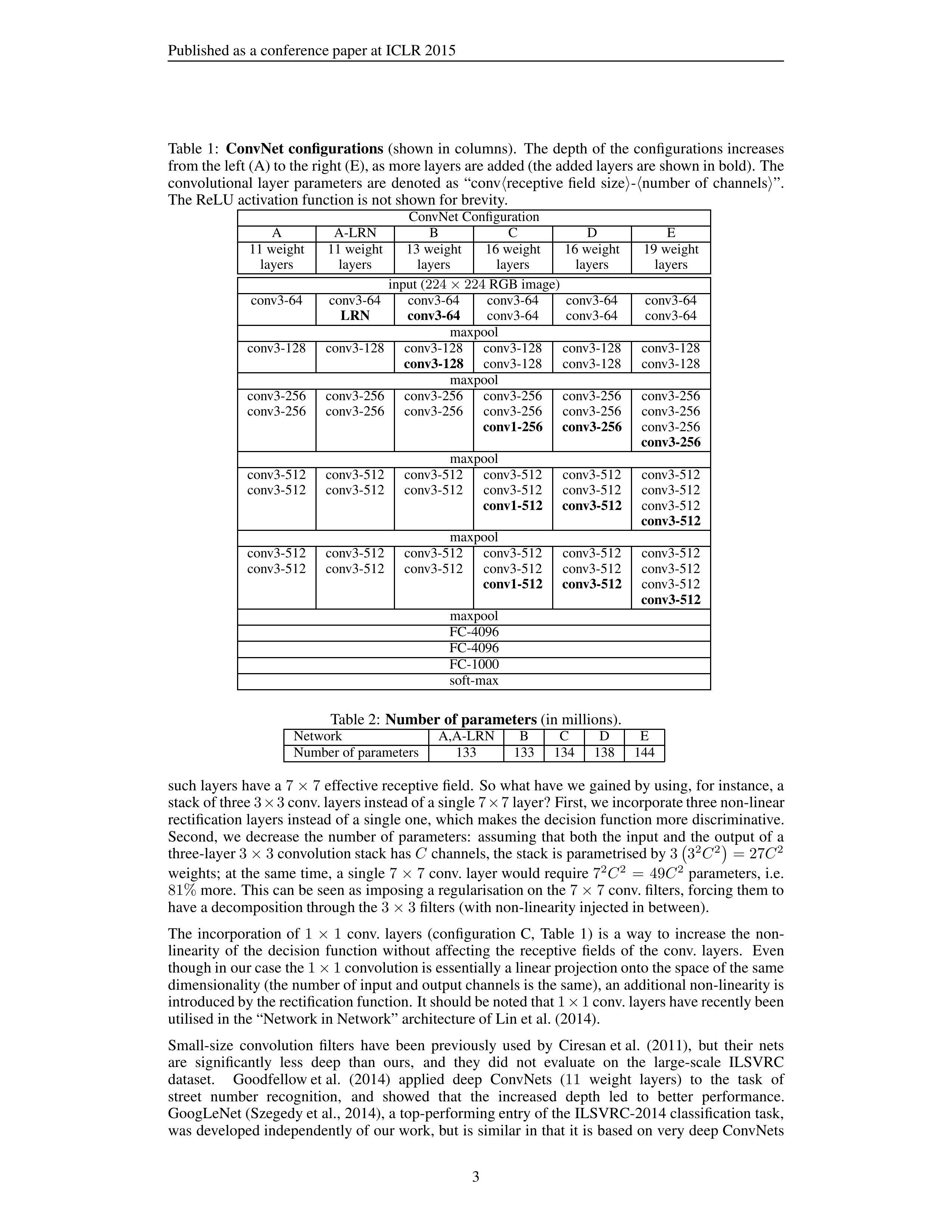
the following we will refer to the nets by their names (A–E). All configurations follow the generic
design presented in Sect. 2.1, and differ only in the depth:
from 11 weight layers in the network A
(8 conv. and 3 FC layers) to 19 weight layers in the network E (16 conv. and 3 FC layers). The width
of conv. layers (the number of channels) is rather small, starting from
64
in the first layer and then
increasing by a factor of
2
after each max-pooling layer, until it reaches
512
.
In Table 2 we report the number of parameters for each configuration.
In spite of a large depth, the
number of weights in our nets is not greater than the number of weights in a more shallow net with
larger conv. layer widths and receptive fields (144M weights in (Sermanet et al., 2014)).
2.3
D
ISCUSSION
Our
ConvNet
configurations
are
quite
different
from
the
ones
used
in
the
top-performing
entries
of
the
ILSVRC-2012
(Krizhevsky et al.,
2012)
and
ILSVRC-2013
competitions
(Zeiler & Fergus,
2013; Sermanet et al., 2014).
Rather than using relatively large receptive fields in the first conv. lay-
ers (e.g.
11
×
11
with stride
4
in (Krizhevsky et al., 2012), or
7
×
7
with stride
2
in (Zeiler & Fergus,
2013;
Sermanet et al.,
2014)),
we
use
very
small
3
×
3
receptive
fields
throughout the
whole
net,
which are convolved with the input at every pixel (with stride
1
). It is easy to see that a stack of two
3
×
3
conv. layers (without spatial pooling in between) has an effective receptive field of
5
×
5
; three
2
Published as a conference paper at ICLR 2015
Table
1:
ConvNet configurations
(shown in
columns).
The
depth
of
the
configurations increases
from the left (A) to the right (E), as more layers are added (the added layers are shown in bold). The
convolutional
layer
parameters
are
denoted
as
“conv
⟨
receptive
field
size
⟩
-
⟨
number
of
channels
⟩
”.
The ReLU activation function is not shown for brevity.
ConvNet Configuration
A
A-LRN
B
C
D
E
11 weight
11 weight
13 weight
16 weight
16 weight
19 weight
layers
layers
layers
layers
layers
layers
input (
224
×
224
RGB image)
conv3-64
conv3-64
conv3-64
conv3-64
conv3-64
conv3-64
LRN
conv3-64
conv3-64
conv3-64
conv3-64
maxpool
conv3-128
conv3-128
conv3-128
conv3-128
conv3-128
conv3-128
conv3-128
conv3-128
conv3-128
conv3-128
maxpool
conv3-256
conv3-256
conv3-256
conv3-256
conv3-256
conv3-256
conv3-256
conv3-256
conv3-256
conv3-256
conv3-256
conv3-256
conv1-256
conv3-256
conv3-256
conv3-256
maxpool
conv3-512
conv3-512
conv3-512
conv3-512
conv3-512
conv3-512
conv3-512
conv3-512
conv3-512
conv3-512
conv3-512
conv3-512
conv1-512
conv3-512
conv3-512
conv3-512
maxpool
conv3-512
conv3-512
conv3-512
conv3-512
conv3-512
conv3-512
conv3-512
conv3-512
conv3-512
conv3-512
conv3-512
conv3-512
conv1-512
conv3-512
conv3-512
conv3-512
maxpool
FC-4096
FC-4096
FC-1000
soft-max
Table 2:
Number of parameters
(in millions).
Network
A,A-LRN
B
C
D
E
Number of parameters
133
133
134
138
144
such layers have a
7
×
7
effective receptive field.
So what have we gained by using, for instance, a
stack of three
3
×
3
conv. layers instead of a single
7
×
7
layer? First, we incorporate three non-linear
rectification layers instead of a single one, which makes the decision function more discriminative.
Second,
we
decrease
the
number
of
parameters:
assuming
that
both
the
input
and
the
output
of
a
three-layer
3
×
3
convolution stack has
C
channels, the stack is parametrised by
3
3
2
C
2
= 27
C
2
weights;
at the same time, a single
7
×
7
conv. layer would require
7
2
C
2
=
49
C
2
parameters, i.e.
81%
more.
This can be seen as imposing a regularisation on the
7
×
7
conv. filters, forcing them to
have a decomposition through the
3
×
3
filters (with non-linearity injected in between).
The
incorporation
of
1
×
1
conv.
layers
(configuration
C,
Table
1)
is
a
way
to
increase
the
non-
linearity
of
the
decision
function
without
affecting
the
receptive
fields
of
the
conv.
layers.
Even
though in our case the
1
×
1
convolution is essentially a linear projection onto the space of the same
dimensionality (the number of input and output channels is the same), an additional non-linearity is
introduced by the rectification function. It should be noted that
1
×
1
conv. layers have recently been
utilised in the “Network in Network” architecture of Lin et al. (2014).
Small-size
convolution
filters
have
been
previously
used
by
Ciresan et al.
(2011),
but
their
nets
are
significantly
less
deep
than
ours,
and
they
did
not
evaluate
on
the
large-scale
ILSVRC
dataset.
Goodfellow et al.
(2014)
applied
deep
ConvNets
(
11
weight
layers)
to
the
task
of
street
number
recognition,
and
showed
that
the
increased
depth
led
to
better
performance.
GoogLeNet (Szegedy et al., 2014), a top-performing entry of the ILSVRC-2014 classification task,
was developed independently of our work, but is similar in that it is based on very deep ConvNets
3
Published as a conference paper at ICLR 2015
(22
weight
layers)
and
small
convolution filters
(apart
from
3
×
3
,
they
also
use
1
×
1
and
5
×
5
convolutions).
Their network topology is,
however, more complex than ours,
and the spatial
reso-
lution
of
the
feature
maps
is
reduced
more
aggressively
in
the
first
layers
to
decrease
the
amount
of
computation.
As
will
be
shown
in
Sect.
4.5,
our
model
is
outperforming that
of
Szegedy et al.
(2014) in terms of the single-network classification accuracy.
3
C
LASSIFICATION
F
RAMEWORK
In the previous section we
presented the
details of our network configurations.
In this section,
we
describe the details of classification ConvNet training and evaluation.
3.1
T
RAINING
The
ConvNet
training
procedure
generally
follows
Krizhevsky et al.
(2012)
(except
for
sampling
the input crops from multi-scale training images, as explained later).
Namely, the training is carried
out
by
optimising
the
multinomial
logistic
regression
objective
using
mini-batch
gradient
descent
(based on back-propagation (LeCun et al., 1989)) with momentum.
The batch size was set
to
256
,
momentum to
0
.
9
.
The
training was
regularised by weight decay (the
L
2
penalty multiplier set
to
5
·
10
−
4
) and dropout regularisation for the first two fully-connected layers (dropout ratio set to
0
.
5
).
The learning rate was initially set to
10
−
2
, and then decreased by a factor of
10
when the validation
set accuracy stopped improving.
In total, the learning rate was decreased 3 times, and the learning
was stopped after
370
K iterations (74 epochs).
We conjecture that in spite of the larger number of
parameters and the greater depth of our nets compared to (Krizhevsky et al., 2012), the nets required
less epochs to converge due to (a) implicit regularisation imposed by greater depth and smaller conv.
filter sizes; (b) pre-initialisation of certain layers.
The initialisation of the network weights is important, since bad initialisation can stall learning due
to
the
instability
of
gradient
in
deep
nets.
To
circumvent
this
problem,
we
began
with
training
the configuration A (Table 1), shallow enough to be trained with random initialisation.
Then, when
training deeper architectures, we initialised the first four convolutional layers and the last three fully-
connected layers with the layers of net A (the intermediate layers were initialised randomly). We did
not decrease the learning rate for the pre-initialised layers, allowing them to change during learning.
For
random
initialisation
(where
applicable),
we
sampled
the
weights
from
a
normal
distribution
with the zero mean and
10
−
2
variance. The biases were initialised with zero.
It is worth noting that
after the paper submission we found that it is possible to initialise the weights without pre-training
by using the random initialisation procedure of Glorot & Bengio (2010).
To obtain the fixed-size
224
×
224
ConvNet input images, they were randomly cropped from rescaled
training
images
(one
crop
per
image
per
SGD
iteration).
To
further
augment
the
training
set,
the
crops underwent random horizontal flipping and random RGB colour shift (Krizhevsky et al., 2012).
Training image rescaling is explained below.
Training image size.
Let
S
be the smallest side of an isotropically-rescaled training image, from
which the ConvNet input is cropped (we also refer to
S
as the training scale).
While the crop size
is fixed to
224
×
224
, in principle
S
can take on any value not less than
224
:
for
S
=
224
the crop
will
capture whole-image statistics,
completely spanning the smallest
side of a
training image;
for
S
≫
224
the crop will correspond to a small part of the image, containing a small object or an object
part.
We consider two approaches for setting the training scale
S
.
The first is to fix
S
, which corresponds
to single-scale training (note that image content within the sampled crops can still represent multi-
scale
image
statistics).
In
our experiments,
we
evaluated models trained at
two
fixed
scales:
S
=
256
(which
has
been
widely
used
in
the
prior
art
(Krizhevsky et al.,
2012;
Zeiler & Fergus,
2013;
Sermanet et al., 2014)) and
S
=
384
.
Given a ConvNet configuration, we first trained the network
using
S
=
256
.
To
speed-up training of
the
S
=
384
network, it
was initialised
with
the
weights
pre-trained with
S
= 256
, and we used a smaller initial learning rate of
10
−
3
.
The second approach to setting
S
is multi-scale training, where each training image is individually
rescaled
by
randomly
sampling
S
from
a
certain
range
[
S
min
, S
max
]
(we
used
S
min
=
256
and
S
max
= 512
). Since objects in images can be of different size, it is beneficial to take this into account
during training. This can also be seen as training set augmentation by scale jittering, where a single
4
Published as a conference paper at ICLR 2015
model
is
trained
to
recognise
objects
over
a
wide
range
of
scales.
For
speed
reasons,
we
trained
multi-scale
models
by
fine-tuning
all
layers
of
a
single-scale
model
with
the
same
configuration,
pre-trained with fixed
S
= 384
.
3.2
T
ESTING
At test time, given a trained ConvNet and an input image, it is classified in the following way. First,
it
is
isotropically
rescaled
to
a
pre-defined
smallest
image
side,
denoted
as
Q
(we
also
refer
to
it
as the test
scale).
We
note that
Q
is not necessarily equal to the training scale
S
(as we will
show
in Sect. 4, using several values of
Q
for each
S
leads to improved performance). Then, the network
is applied densely over the rescaled test image in a way similar to (Sermanet et al., 2014).
Namely,
the
fully-connected layers are
first
converted to
convolutional layers
(the
first
FC
layer
to
a
7
×
7
conv. layer,
the
last
two
FC
layers
to
1
×
1
conv. layers).
The
resulting
fully-convolutional net
is
then
applied to
the
whole
(uncropped) image.
The
result
is
a
class
score
map
with
the
number of
channels equal
to
the
number of
classes,
and
a
variable
spatial
resolution,
dependent on
the
input
image size.
Finally, to obtain a fixed-size vector of class scores for the image, the class score map is
spatially averaged (sum-pooled).
We also augment the test set by horizontal flipping of the images;
the soft-max class posteriors of the original and flipped images are averaged to obtain the final scores
for the image.
Since the
fully-convolutional network is
applied over the whole image, there is no need to
sample
multiple
crops
at
test
time
(Krizhevsky et al.,
2012),
which
is
less
efficient
as
it
requires
network
re-computation for each crop. At the same time, using a large set of crops, as done by Szegedy et al.
(2014), can lead to improved accuracy, as it results in a finer sampling of the input image compared
to the fully-convolutional net. Also, multi-crop evaluation is complementary to dense evaluation due
to
different convolution boundary conditions:
when
applying
a
ConvNet
to
a
crop,
the
convolved
feature maps are padded with zeros, while in the case of dense evaluation the padding for the same
crop
naturally
comes
from
the
neighbouring parts
of
an
image
(due
to
both
the
convolutions and
spatial pooling), which substantially increases the overall network receptive field,
so
more context
is captured. While we believe that in practice the increased computation time of multiple crops does
not justify the potential gains in accuracy, for reference we also evaluate our networks using
50
crops
per scale (
5
×
5
regular grid with
2
flips), for a total of
150
crops over
3
scales, which is comparable
to
144
crops over
4
scales used by Szegedy et al. (2014).
3.3
I
MPLEMENTATION
D
ETAILS
Our implementation is derived from the publicly available C++ Caffe toolbox (Jia, 2013) (branched
out in December 2013), but contains a number of significant modifications, allowing us to perform
training and evaluation on multiple GPUs installed in a single system, as well as train and evaluate on
full-size
(uncropped) images at
multiple scales
(as described above).
Multi-GPU
training exploits
data
parallelism,
and
is
carried
out
by
splitting
each
batch
of
training
images
into
several
GPU
batches, processed in parallel on each GPU. After the GPU batch gradients are computed, they are
averaged to
obtain the
gradient of
the
full
batch.
Gradient computation is
synchronous across
the
GPUs, so the result is exactly the same as when training on a single GPU.
While
more
sophisticated
methods
of
speeding
up
ConvNet
training
have
been
recently
pro-
posed (Krizhevsky, 2014), which employ model and data parallelism for different layers of the net,
we have found that our conceptually much simpler scheme already provides a speedup of
3
.
75
times
on an off-the-shelf 4-GPU system, as compared to using a single GPU. On a system equipped with
four NVIDIA Titan Black GPUs, training a single net took 2–3 weeks depending on the architecture.
4
C
LASSIFICATION
E
XPERIMENTS
Dataset.
In
this
section,
we
present
the
image
classification
results
achieved
by
the
described
ConvNet architectures on the ILSVRC-2012 dataset (which was used for ILSVRC 2012–2014 chal-
lenges).
The
dataset
includes
images
of
1000
classes,
and
is
split
into
three
sets:
training
(
1
.
3
M
images), validation (
50
K images), and testing (
100
K images with held-out class labels).
The clas-
sification performance is evaluated using two measures:
the top-1 and top-5 error.
The former is a
multi-class
classification
error,
i.e.
the
proportion of
incorrectly classified
images;
the
latter
is
the
5
Published as a conference paper at ICLR 2015
main evaluation criterion used in ILSVRC,
and is computed as
the proportion of images such that
the ground-truth category is outside the top-5 predicted categories.
For the majority of experiments, we used the validation set as the test set.
Certain experiments were
also carried out on the test set and submitted to the official ILSVRC server as a “VGG” team entry
to the ILSVRC-2014 competition (Russakovsky et al., 2014).
4.1
S
INGLE
S
CALE
E
VALUATION
We begin with evaluating the performance of individual ConvNet models at a single scale with the
layer configurations described in Sect. 2.2.
The test image size was set as follows:
Q
=
S
for fixed
S
, and
Q
= 0
.
5(
S
min
+
S
max
)
for jittered
S
∈
[
S
min
, S
max
]
.
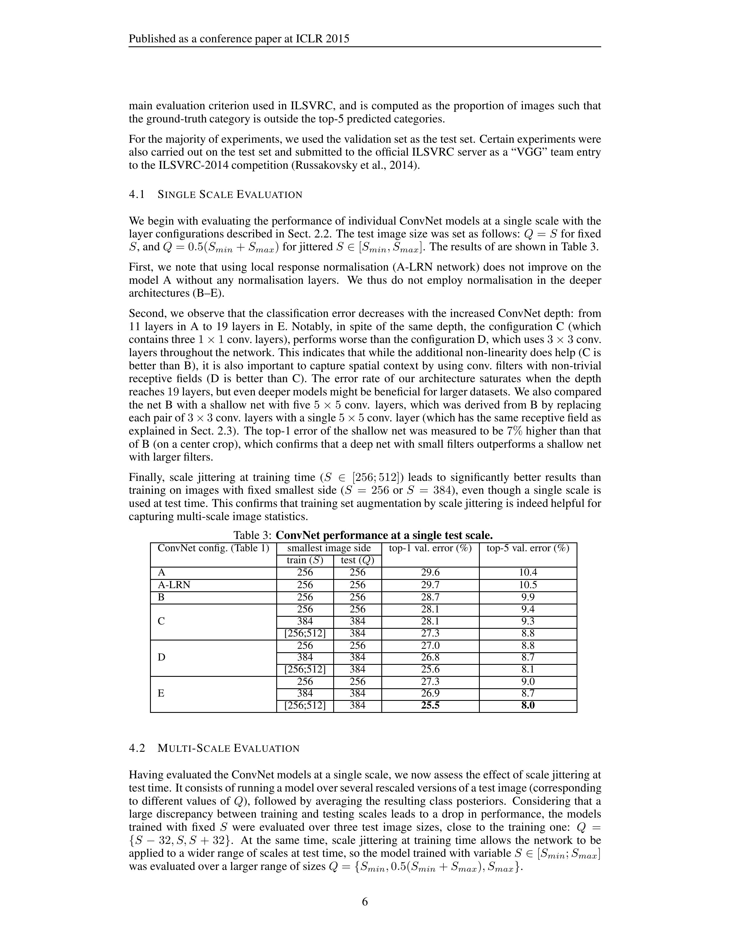
The results of are shown in Table 3.
First,
we
note
that
using
local
response
normalisation
(A-LRN
network)
does
not
improve on
the
model
A
without
any
normalisation
layers.
We
thus
do
not
employ
normalisation
in
the
deeper
architectures (B–E).
Second, we observe that the classification error decreases with the increased ConvNet depth:
from
11
layers
in
A
to
19
layers
in
E.
Notably,
in
spite
of
the
same
depth,
the
configuration C
(which
contains three
1
×
1
conv. layers), performs worse than the configuration D, which uses
3
×
3
conv.
layers throughout the network. This indicates that while the additional non-linearity does help (C is
better
than
B),
it
is
also
important to
capture
spatial
context
by
using conv. filters
with
non-trivial
receptive
fields
(D
is
better
than
C).
The
error
rate
of
our
architecture
saturates
when
the
depth
reaches
19
layers, but even deeper models might be beneficial for larger datasets.
We also compared
the net
B with a
shallow net
with five
5
×
5
conv.
layers,
which was derived from B by replacing
each pair of
3
×
3
conv. layers with a single
5
×
5
conv. layer (which has the same receptive field as
explained in Sect. 2.3).
The top-1 error of the shallow net was measured to be
7%
higher than that
of B (on a center crop), which confirms that a deep net with small filters outperforms a shallow net
with larger filters.
Finally,
scale
jittering
at
training
time
(
S
∈
[256; 512]
)
leads
to
significantly
better
results
than
training
on
images with
fixed
smallest
side
(
S
=
256
or
S
=
384
),
even
though a
single
scale
is
used at test time.
This confirms that training set augmentation by scale jittering is indeed helpful for
capturing multi-scale image statistics.
Table 3:
ConvNet performance at a single test scale.
ConvNet config. (Table 1)
smallest image side
top-1 val. error (%)
top-5 val. error (%)
train (
S
)
test (
Q
)
A
256
256
29.6
10.4
A-LRN
256
256
29.7
10.5
B
256
256
28.7
9.9
C
256
256
28.1
9.4
384
384
28.1
9.3
[256;512]
384
27.3
8.8
D
256
256
27.0
8.8
384
384
26.8
8.7
[256;512]
384
25.6
8.1
E
256
256
27.3
9.0
384
384
26.9
8.7
[256;512]
384
25.5
8.0
4.2
M
ULTI
-S
CALE
E
VALUATION
Having evaluated the ConvNet models at a single scale, we now assess the effect of scale jittering at
test time. It consists of running a model over several rescaled versions of a test image (corresponding
to
different values
of
Q
),
followed by
averaging the
resulting
class
posteriors.
Considering that
a
large
discrepancy
between
training
and
testing
scales
leads
to
a
drop
in
performance,
the
models
trained
with
fixed
S
were
evaluated
over
three
test
image
sizes,
close
to
the
training
one:
Q
=
{
S
−
32
, S, S
+ 32
}
.
At
the
same
time,
scale
jittering
at
training
time
allows
the
network
to
be
applied to a wider range of scales at test time, so the model trained with variable
S
∈
[
S
min
;
S
max
]
was evaluated over a larger range of sizes
Q
=
{
S
min
,
0
.
5(
S
min
+
S
max
)
, S
max
}
.
6
Published as a conference paper at ICLR 2015
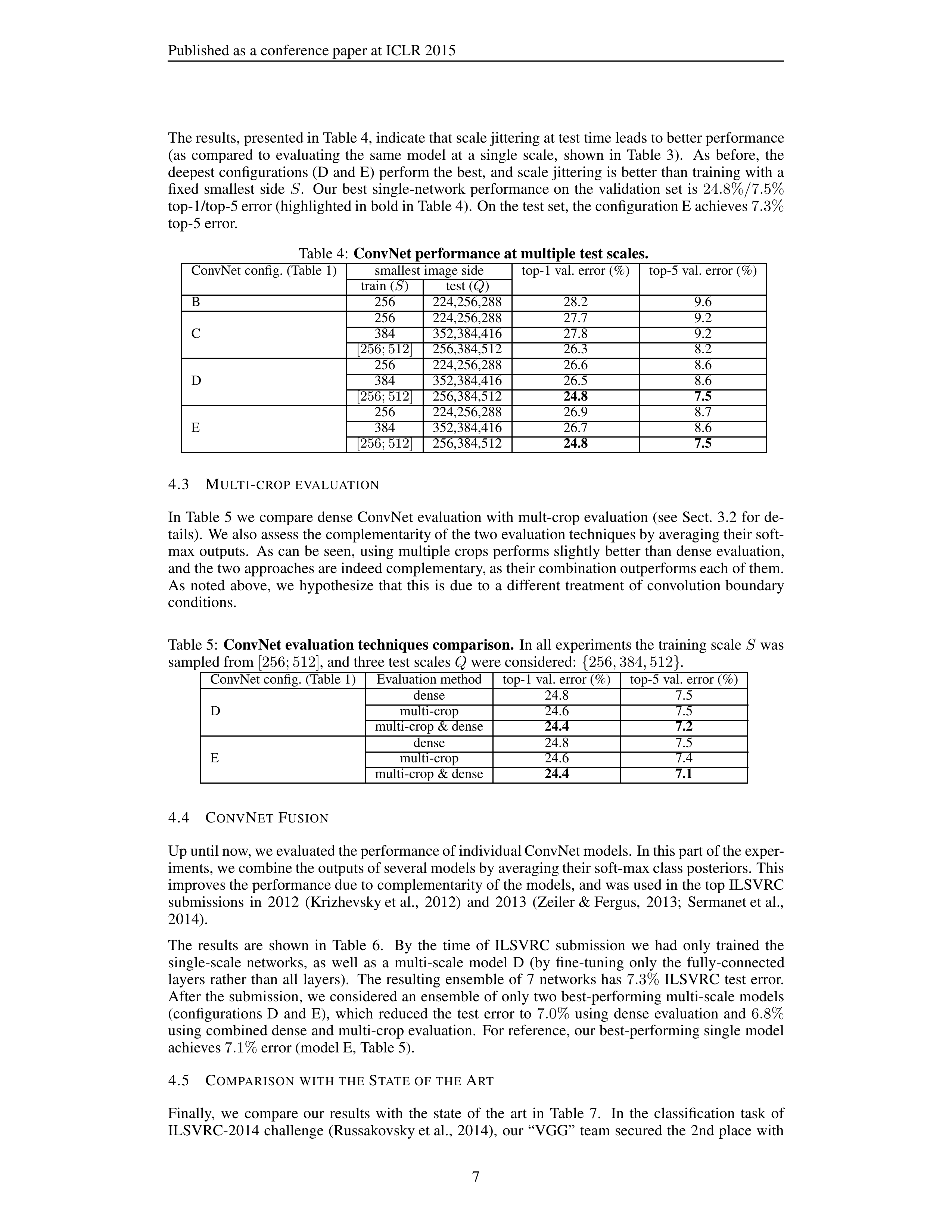
The results, presented in Table 4, indicate that scale jittering at test time leads to better performance
(as
compared
to
evaluating
the
same
model
at
a
single
scale,
shown
in
Table
3).
As
before,
the
deepest configurations (D and E) perform the best,
and scale jittering is better than training with a
fixed
smallest
side
S
.
Our
best
single-network
performance on
the
validation
set
is
24
.
8%
/
7
.
5%
top-1/top-5 error (highlighted in bold in Table 4).
On the test set, the configuration E achieves
7
.
3%
top-5 error.
Table 4:
ConvNet performance at multiple test scales.
ConvNet config. (Table 1)
smallest image side
top-1 val. error (%)
top-5 val. error (%)
train (
S
)
test (
Q
)
B
256
224,256,288
28.2
9.6
C
256
224,256,288
27.7
9.2
384
352,384,416
27.8
9.2
[256; 512]
256,384,512
26.3
8.2
D
256
224,256,288
26.6
8.6
384
352,384,416
26.5
8.6
[256; 512]
256,384,512
24.8
7.5
E
256
224,256,288
26.9
8.7
384
352,384,416
26.7
8.6
[256; 512]
256,384,512
24.8
7.5
4.3
M
ULTI
-
CROP
EVALUATION
In Table
5 we
compare dense ConvNet evaluation with mult-crop evaluation (see Sect.
3.2 for de-
tails).
We also assess the complementarity of the two evaluation techniques by averaging their soft-
max outputs.
As can
be seen,
using multiple crops performs slightly
better than dense
evaluation,
and the two approaches are indeed complementary, as their combination outperforms each of them.
As
noted
above,
we
hypothesize
that
this
is
due
to
a
different
treatment
of
convolution boundary
conditions.
Table 5:
ConvNet evaluation techniques comparison.
In all experiments the training scale
S
was
sampled from
[256; 512]
, and three test scales
Q
were considered:
{
256
,
384
,
512
}
.
ConvNet config. (Table 1)
Evaluation method
top-1 val. error (%)
top-5 val. error (%)
D
dense
24.8
7.5
multi-crop
24.6
7.5
multi-crop & dense
24.4
7.2
E
dense
24.8
7.5
multi-crop
24.6
7.4
multi-crop & dense
24.4
7.1
4.4
C
ONV
N
ET
F
USION
Up until now, we evaluated the performance of individual ConvNet models. In this part of the exper-
iments, we combine the outputs of several models by averaging their soft-max class posteriors. This
improves the performance due to complementarity of the models, and was used in the top ILSVRC
submissions
in
2012
(Krizhevsky et al.,
2012)
and
2013
(Zeiler & Fergus,
2013;
Sermanet et al.,
2014).
The
results
are
shown
in
Table
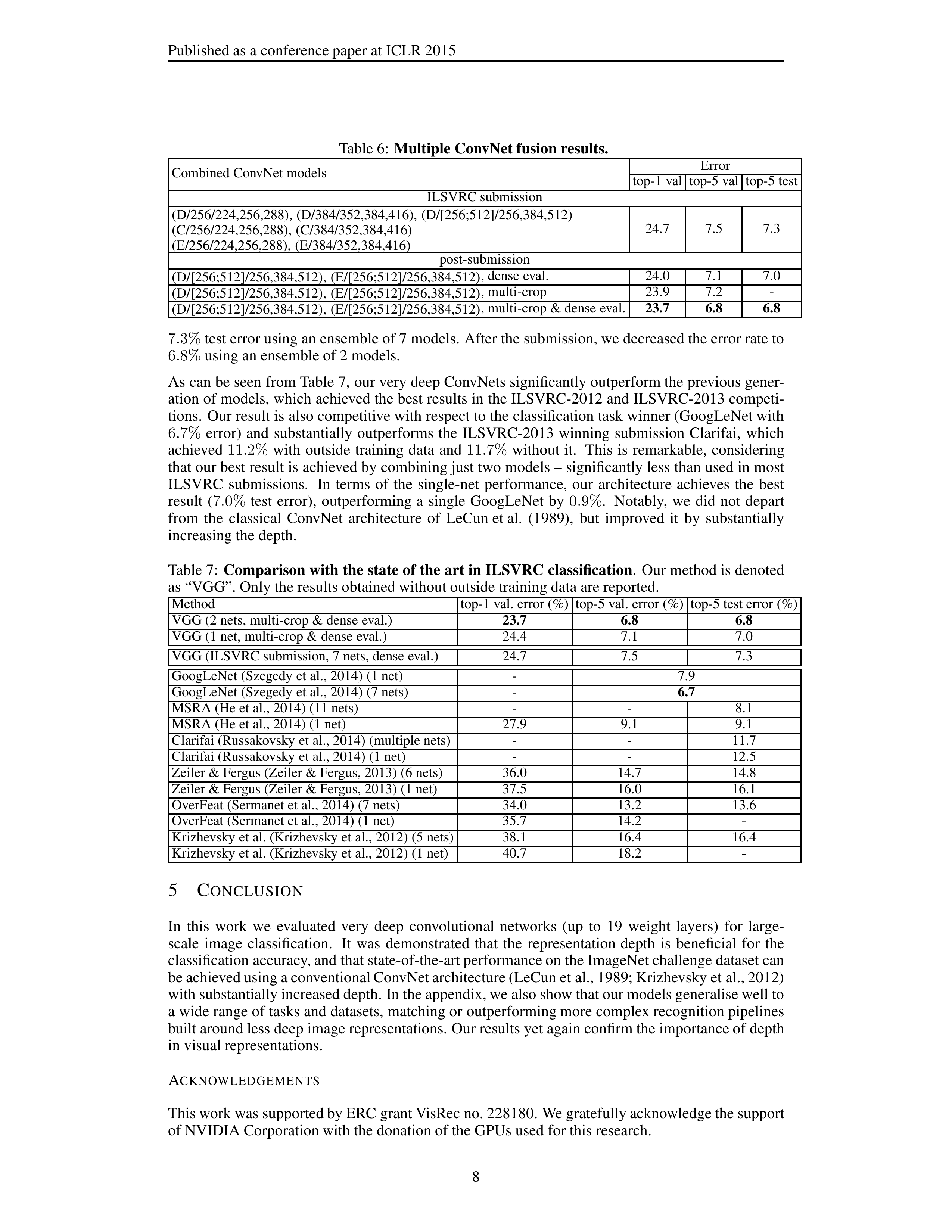
6.
By
the
time
of
ILSVRC
submission
we
had
only
trained
the
single-scale
networks,
as
well
as
a
multi-scale
model
D
(by
fine-tuning
only
the
fully-connected
layers
rather
than
all
layers).
The
resulting
ensemble
of
7
networks has
7
.
3%
ILSVRC
test
error.
After the submission, we considered an ensemble of only two best-performing multi-scale models
(configurations D
and
E),
which
reduced
the
test
error
to
7
.
0%
using
dense
evaluation
and
6
.
8%
using combined dense and multi-crop evaluation.
For reference, our best-performing single model
achieves
7
.
1%
error (model E, Table 5).
4.5
C
OMPARISON
WITH
THE
S
TATE
OF
THE
A
RT
Finally,
we
compare
our
results
with
the
state
of
the
art
in
Table
7.
In
the
classification
task
of
ILSVRC-2014 challenge (Russakovsky et al.,
2014),
our “VGG”
team
secured the
2nd place
with
7
Published as a conference paper at ICLR 2015
Table 6:
Multiple ConvNet fusion results.
Combined ConvNet models
Error
top-1 val
top-5 val
top-5 test
ILSVRC submission
(D/256/224,256,288), (D/384/352,384,416), (D/[256;512]/256,384,512)
(C/256/224,256,288), (C/384/352,384,416)
(E/256/224,256,288), (E/384/352,384,416)
24.7
7.5
7.3
post-submission
(D/[256;512]/256,384,512), (E/[256;512]/256,384,512), dense eval.
24.0
7.1
7.0
(D/[256;512]/256,384,512), (E/[256;512]/256,384,512)
, multi-crop
23.9
7.2
-
(D/[256;512]/256,384,512), (E/[256;512]/256,384,512), multi-crop & dense eval.
23.7
6.8
6.8
7
.
3%
test error using an ensemble of 7 models. After the submission, we decreased the error rate to
6
.
8%
using an ensemble of 2 models.
As can be seen from Table 7, our very deep ConvNets significantly outperform the previous gener-
ation of models, which achieved the best results in the ILSVRC-2012 and ILSVRC-2013 competi-
tions.
Our result is also competitive with respect to the classification task winner (GoogLeNet with
6
.
7%
error)
and
substantially
outperforms the
ILSVRC-2013
winning
submission
Clarifai,
which
achieved
11
.
2%
with
outside
training
data
and
11
.
7%
without
it.
This
is
remarkable,
considering
that our best result is achieved by combining just two models – significantly less than used in most
ILSVRC
submissions.
In
terms
of
the
single-net
performance,
our
architecture
achieves
the
best
result
(
7
.
0%
test
error),
outperforming a
single
GoogLeNet
by
0
.
9%
.
Notably,
we
did
not
depart
from
the
classical
ConvNet
architecture
of
LeCun et al.
(1989),
but
improved
it
by
substantially
increasing the depth.
Table 7:
Comparison with the state of the art in ILSVRC classification
.
Our method is denoted
as “VGG”. Only the results obtained without outside training data are reported.
Method
top-1 val. error (%)
top-5 val. error (%)
top-5 test error (%)
VGG (2 nets, multi-crop & dense eval.)
23.7
6.8
6.8
VGG (1 net, multi-crop & dense eval.)
24.4
7.1
7.0
VGG (ILSVRC submission, 7 nets, dense eval.)
24.7
7.5
7.3
GoogLeNet (Szegedy et al., 2014) (1 net)
-
7.9
GoogLeNet (Szegedy et al., 2014) (7 nets)
-
6.7
MSRA (He et al., 2014) (11 nets)
-
-
8.1
MSRA (He et al., 2014) (1 net)
27.9
9.1
9.1
Clarifai (Russakovsky et al., 2014) (multiple nets)
-
-
11.7
Clarifai (Russakovsky et al., 2014) (1 net)
-
-
12.5
Zeiler & Fergus (Zeiler & Fergus, 2013) (6 nets)
36.0
14.7
14.8
Zeiler & Fergus (Zeiler & Fergus, 2013) (1 net)
37.5
16.0
16.1
OverFeat (Sermanet et al., 2014) (7 nets)
34.0
13.2
13.6
OverFeat (Sermanet et al., 2014) (1 net)
35.7
14.2
-
Krizhevsky et al. (Krizhevsky et al., 2012) (5 nets)
38.1
16.4
16.4
Krizhevsky et al. (Krizhevsky et al., 2012) (1 net)
40.7
18.2
-
5
C
ONCLUSION
In
this
work
we
evaluated
very
deep
convolutional
networks
(up
to
19
weight
layers)
for
large-
scale
image
classification.
It
was
demonstrated
that
the
representation
depth
is
beneficial
for
the
classification accuracy, and that state-of-the-art performance on the ImageNet challenge dataset can
be achieved using a conventional ConvNet architecture (LeCun et al., 1989; Krizhevsky et al., 2012)
with substantially increased depth. In the appendix, we also show that our models generalise well to
a wide range of tasks and datasets, matching or outperforming more complex recognition pipelines
built around less deep image representations. Our results yet again confirm the importance of depth
in visual representations.
A
CKNOWLEDGEMENTS
This work was supported by ERC grant VisRec no. 228180. We gratefully acknowledge the support
of NVIDIA Corporation with the donation of the GPUs used for this research.
8
Published as a conference paper at ICLR 2015
R
EFERENCES
Bell, S., Upchurch, P., Snavely, N., and Bala, K.
Material recognition in the wild with the materials in context
database.
CoRR
, abs/1412.0623, 2014.
Chatfield,
K., Simonyan,
K., Vedaldi,
A., and
Zisserman,
A.
Return
of the devil
in the details:
Delving
deep
into convolutional nets.
In
Proc. BMVC.
, 2014.
Cimpoi, M., Maji, S., and Vedaldi, A. Deep convolutional filter banks for texture recognition and segmentation.
CoRR
, abs/1411.6836, 2014.
Ciresan,
D.
C.,
Meier,
U.,
Masci,
J.,
Gambardella,
L.
M.,
and
Schmidhuber,
J.
Flexible,
high
performance
convolutional neural networks for image classification.
In
IJCAI
, pp. 1237–1242, 2011.
Dean,
J., Corrado,
G.,
Monga,
R., Chen,
K.,
Devin,
M.,
Mao,
M.,
Ranzato,
M.,
Senior,
A.,
Tucker,
P., Yang,
K., Le, Q. V., and Ng, A. Y.
Large scale distributed deep networks.
In
NIPS
, pp. 1232–1240, 2012.
Deng,
J.,
Dong,
W.,
Socher,
R.,
Li,
L.-J.,
Li, K.,
and
Fei-Fei, L.
Imagenet:
A
large-scale
hierarchical
image
database.
In
Proc. CVPR
, 2009.
Donahue, J., Jia, Y., Vinyals, O., Hoffman, J., Zhang, N., Tzeng, E., and Darrell, T. Decaf: A deep convolutional
activation feature for generic visual recognition.
CoRR
, abs/1310.1531, 2013.
Everingham, M., Eslami, S. M. A., Van Gool, L., Williams, C., Winn, J., and Zisserman, A.
The Pascal visual
object classes challenge:
A retrospective.
IJCV
, 111(1):98–136, 2015.
Fei-Fei,
L.,
Fergus,
R.,
and
Perona,
P.
Learning
generative
visual
models
from
few
training
examples:
An
incremental
bayesian
approach
tested
on
101
object
categories.
In
IEEE
CVPR
Workshop
of
Generative
Model Based Vision
, 2004.
Girshick,
R. B., Donahue,
J.,
Darrell,
T.,
and
Malik,
J.
Rich
feature
hierarchies
for
accurate
object
detection
and semantic segmentation.
CoRR
, abs/1311.2524v5, 2014.
Published in Proc. CVPR, 2014.
Gkioxari, G., Girshick, R., and Malik, J.
Actions and attributes from wholes and parts.
CoRR
, abs/1412.2604,
2014.
Glorot, X. and Bengio, Y.
Understanding the difficulty of training deep feedforward neural networks.
In
Proc.
AISTATS
, volume 9, pp. 249–256, 2010.
Goodfellow,
I.
J.,
Bulatov,
Y.,
Ibarz,
J.,
Arnoud,
S.,
and
Shet,
V.
Multi-digit
number
recognition
from
street
view imagery using deep convolutional neural networks.
In
Proc. ICLR
, 2014.
Griffin, G., Holub, A., and Perona, P.
Caltech-256 object category dataset.
Technical Report 7694, California
Institute of Technology, 2007.
He,
K.,
Zhang,
X.,
Ren,
S.,
and
Sun,
J.
Spatial
pyramid
pooling
in
deep
convolutional
networks
for
visual
recognition.
CoRR
, abs/1406.4729v2, 2014.
Hoai, M.
Regularized max pooling for image categorization.
In
Proc. BMVC.
, 2014.
Howard, A. G.
Some improvements on deep convolutional neural network based image classification.
In
Proc.
ICLR
, 2014.
Jia,
Y.
Caffe:
An
open
source
convolutional
architecture
for
fast
feature
embedding.
http://caffe.berkeleyvision.org/
, 2013.
Karpathy,
A.
and
Fei-Fei,
L.
Deep
visual-semantic
alignments
for
generating
image
descriptions.
CoRR
,
abs/1412.2306, 2014.
Kiros, R., Salakhutdinov, R., and Zemel, R. S.
Unifying visual-semantic embeddings
with multimodal neural
language models.
CoRR
, abs/1411.2539, 2014.
Krizhevsky, A.
One weird trick for parallelizing convolutional neural networks.
CoRR
, abs/1404.5997, 2014.
Krizhevsky,
A.,
Sutskever,
I.,
and
Hinton,
G.
E.
ImageNet
classification
with
deep
convolutional
neural
net-
works.
In
NIPS
, pp. 1106–1114, 2012.
LeCun, Y., Boser, B., Denker, J. S., Henderson, D., Howard, R. E., Hubbard, W., and Jackel, L. D.
Backpropa-
gation applied to handwritten zip code recognition.
Neural Computation
, 1(4):541–551, 1989.
Lin, M., Chen, Q., and Yan, S.
Network in network.
In
Proc. ICLR
, 2014.
Long,
J.,
Shelhamer,
E.,
and
Darrell,
T.
Fully
convolutional
networks
for
semantic
segmentation.
CoRR
,
abs/1411.4038, 2014.
Oquab,
M.,
Bottou,
L., Laptev,
I., and
Sivic, J.
Learning
and
Transferring
Mid-Level
Image
Representations
using Convolutional Neural Networks.
In
Proc. CVPR
, 2014.
Perronnin, F., S´anchez, J., and Mensink, T.
Improving the Fisher kernel for large-scale image classification.
In
Proc. ECCV
, 2010.
Razavian, A., Azizpour, H., Sullivan, J., and Carlsson, S.
CNN Features off-the-shelf:
an Astounding Baseline
for Recognition.
CoRR
, abs/1403.6382, 2014.
9
Published as a conference paper at ICLR 2015
Russakovsky,
O.,
Deng,
J.,
Su,
H.,
Krause,
J.,
Satheesh,
S.,
Ma,
S.,
Huang,
Z.,
Karpathy,
A.,
Khosla,
A.,
Bernstein,
M.,
Berg,
A.
C.,
and
Fei-Fei,
L.
ImageNet
large
scale
visual
recognition
challenge.
CoRR
,
abs/1409.0575, 2014.
Sermanet, P., Eigen, D., Zhang, X., Mathieu, M., Fergus, R., and LeCun, Y.
OverFeat:
Integrated Recognition,
Localization and Detection using Convolutional Networks.
In
Proc. ICLR
, 2014.
Simonyan, K. and Zisserman, A.
Two-stream convolutional networks for action recognition in videos.
CoRR
,
abs/1406.2199, 2014.
Published in Proc. NIPS, 2014.
Szegedy, C., Liu, W., Jia, Y., Sermanet, P., Reed, S., Anguelov, D., Erhan, D., Vanhoucke, V., and Rabinovich,
A.
Going deeper with convolutions.
CoRR
, abs/1409.4842, 2014.
Wei, Y., Xia, W., Huang, J., Ni, B., Dong, J., Zhao, Y., and Yan, S.
CNN: Single-label to multi-label.
CoRR
,
abs/1406.5726, 2014.
Zeiler,
M.
D.
and
Fergus,
R.
Visualizing
and
understanding
convolutional
networks.
CoRR
,
abs/1311.2901,
2013.
Published in Proc. ECCV, 2014.
A
L
OCALISATION
In the main body of the paper we have considered the classification task of the ILSVRC challenge,
and
performed a
thorough evaluation of
ConvNet
architectures of
different depth.
In
this
section,
we
turn to the localisation task of the challenge, which we have won in
2014 with
25
.
3%
error.
It
can
be
seen
as
a
special
case
of
object
detection,
where
a
single
object
bounding
box
should
be
predicted for each of the top-5 classes, irrespective of the actual number of objects of the class.
For
this we adopt the approach of Sermanet et al. (2014), the winners of the ILSVRC-2013 localisation
challenge, with a few modifications. Our method is described in Sect. A.1 and evaluated in Sect. A.2.
A.1
L
OCALISATION
C
ONV
N
ET
To
perform object
localisation,
we
use
a
very
deep
ConvNet,
where
the
last
fully
connected layer
predicts the
bounding box
location
instead
of
the
class
scores.
A
bounding box
is
represented by
a
4-D
vector
storing
its
center
coordinates,
width,
and
height.
There
is
a
choice
of
whether
the
bounding box prediction is shared across all classes (single-class regression, SCR (Sermanet et al.,
2014)) or is class-specific (per-class regression, PCR). In the former case, the last layer is 4-D, while
in the latter it is 4000-D (since there are 1000 classes in the dataset).
Apart from the last bounding
box prediction layer, we use the ConvNet architecture D (Table 1), which contains 16 weight layers
and was found to be the best-performing in the classification task (Sect. 4).
Training.
Training
of
localisation
ConvNets
is
similar
to
that
of
the
classification
ConvNets
(Sect. 3.1).
The main difference is that we replace the logistic regression objective with a Euclidean
loss, which penalises the deviation of the predicted bounding box parameters from the ground-truth.
We trained two localisation models, each on a single scale:
S
=
256
and
S
=
384
(due to the time
constraints, we did not use training scale jittering for our ILSVRC-2014 submission).
Training was
initialised with the corresponding classification models (trained on the same scales), and the initial
learning rate was set to
10
−
3
.
We explored both fine-tuning all layers and fine-tuning only the first
two
fully-connected layers,
as done in
(Sermanet et al.,
2014).
The
last
fully-connected layer
was
initialised randomly and trained from scratch.
Testing.
We
consider
two
testing
protocols.
The
first
is
used
for
comparing
different
network
modifications on the validation set, and considers only the bounding box prediction for the ground
truth
class
(to
factor
out
the
classification
errors).
The
bounding box
is
obtained
by
applying
the
network only to the central crop of the image.
The
second,
fully-fledged,
testing
procedure
is
based
on
the
dense
application
of
the
localisation
ConvNet to
the
whole image,
similarly to
the
classification
task
(Sect.
3.2).
The difference is that
instead
of
the
class
score
map,
the
output
of
the
last
fully-connected
layer
is
a
set
of
bounding
box
predictions.
To
come
up
with
the
final
prediction,
we
utilise
the
greedy
merging
procedure
of
Sermanet et al.
(2014),
which
first
merges
spatially
close
predictions
(by
averaging
their
coor-
dinates),
and
then
rates
them
based
on
the
class
scores,
obtained from
the
classification
ConvNet.
When several localisation ConvNets are used, we first take the union of their sets of bounding box
predictions, and then run the merging procedure on the union.
We did not use the multiple pooling
10

Published as a conference paper at ICLR 2015
offsets technique of
Sermanet et al.
(2014),
which increases the
spatial
resolution of
the
bounding
box predictions and can further improve the results.
A.2
L
OCALISATION
E
XPERIMENTS
In this section we first determine the best-performing localisation setting (using the first test proto-
col),
and
then
evaluate
it
in
a
fully-fledged
scenario
(the
second
protocol).
The
localisation
error
is
measured
according
to
the
ILSVRC
criterion
(Russakovsky et al.,
2014),
i.e.
the
bounding box
prediction is deemed correct if its intersection over union ratio with the ground-truth bounding box
is above
0
.
5
.
Settings comparison.
As
can be
seen
from Table
8,
per-class regression (PCR)
outperforms the
class-agnostic
single-class
regression
(SCR),
which
differs
from
the
findings
of
Sermanet et al.
(2014),
where PCR
was
outperformed by
SCR.
We
also
note
that
fine-tuning all
layers for
the
lo-
calisation task leads to noticeably better results than fine-tuning only the fully-connected layers (as
done in (Sermanet et al., 2014)).
In these experiments, the smallest images side was set to
S
= 384
;
the results with
S
= 256
exhibit the same behaviour and are not shown for brevity.
Table
8:
Localisation error
for
different
modifications
with
the
simplified
testing
protocol:
the
bounding box is predicted from a single central image crop, and the ground-truth class is used.
All
ConvNet
layers
(except
for
the
last
one)
have
the
configuration
D
(Table
1),
while
the
last
layer
performs either single-class regression (SCR) or per-class regression (PCR).
Fine-tuned layers
regression type
GT class localisation error
1st and 2nd FC
SCR
36.4
PCR
34.3
all
PCR
33.1
Fully-fledged evaluation.
Having determined the best localisation setting (PCR, fine-tuning of all
layers), we now apply it in the fully-fledged scenario, where the top-5 class labels are predicted us-
ing our best-performing classification system (Sect. 4.5), and multiple densely-computed bounding
box
predictions are
merged using
the
method of
Sermanet et al.
(2014).
As
can
be
seen
from
Ta-
ble 9, application of the localisation ConvNet to the whole image substantially improves the results
compared to using a center crop (Table 8), despite using the top-5 predicted class labels instead of
the ground truth. Similarly to the classification task (Sect. 4), testing at several scales and combining
the predictions of multiple networks further improves the performance.
Table 9:
Localisation error
smallest image side
top-5 localisation error (%)
train (
S
)
test (
Q
)
val.
test.
256
256
29.5
-
384
384
28.2
26.7
384
352,384
27.5
-
fusion:
256/256 and 384/352,384
26.9
25.3
Comparison
with
the
state
of
the
art.
We
compare
our
best
localisation
result
with
the
state
of
the
art
in
Table
10.
With
25
.
3%
test
error,
our
“VGG”
team
won
the
localisation
challenge
of
ILSVRC-2014
(Russakovsky et al.,
2014).
Notably,
our
results
are
considerably better
than
those
of the ILSVRC-2013 winner Overfeat (Sermanet et al., 2014), even though we used less scales and
did
not
employ
their
resolution
enhancement technique.
We
envisage
that
better
localisation
per-
formance
can
be
achieved
if
this
technique
is
incorporated
into
our
method.
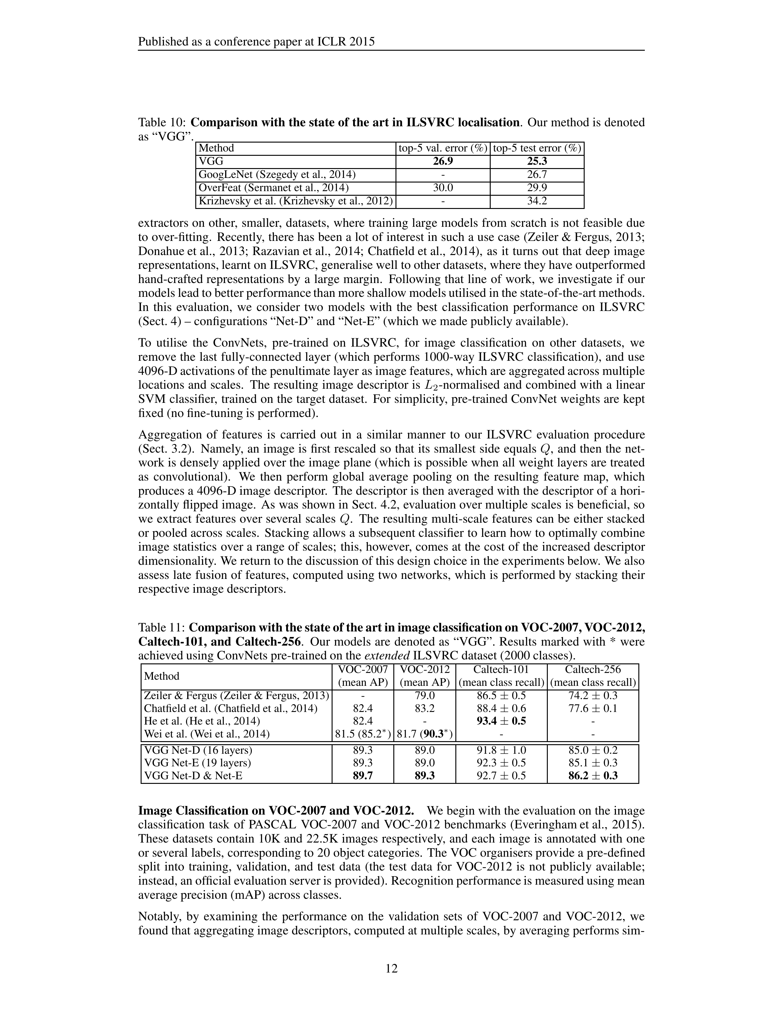
This
indicates
the
performance advancement brought by our very deep ConvNets – we got better results with a simpler
localisation method, but a more powerful representation.
B
G
ENERALISATION
OF
V
ERY
D
EEP
F
EATURES
In
the
previous sections
we
have
discussed
training
and
evaluation
of
very
deep
ConvNets
on
the
ILSVRC
dataset.
In
this
section,
we
evaluate
our
ConvNets,
pre-trained
on
ILSVRC,
as
feature
11
Published as a conference paper at ICLR 2015
Table 10:
Comparison with the state of the art in ILSVRC localisation
.
Our method is denoted
as “VGG”.
Method
top-5 val. error (%)
top-5 test error (%)
VGG
26.9
25.3
GoogLeNet (Szegedy et al., 2014)
-
26.7
OverFeat (Sermanet et al., 2014)
30.0
29.9
Krizhevsky et al. (Krizhevsky et al., 2012)
-
34.2
extractors on other,
smaller,
datasets,
where training large models from scratch is not
feasible due
to over-fitting.
Recently, there has been a lot of interest in such a use case (Zeiler & Fergus, 2013;
Donahue et al.,
2013;
Razavian et al.,
2014;
Chatfield et al.,
2014),
as
it
turns out
that
deep
image
representations, learnt on ILSVRC, generalise well to other datasets, where they have outperformed
hand-crafted representations by
a
large margin.
Following that
line
of
work,
we
investigate if
our
models lead to better performance than more shallow models utilised in the state-of-the-art methods.
In
this
evaluation,
we
consider
two
models
with
the
best
classification
performance
on
ILSVRC
(Sect. 4) – configurations “Net-D” and “Net-E” (which we made publicly available).
To
utilise
the
ConvNets,
pre-trained
on
ILSVRC,
for
image
classification
on
other
datasets,
we
remove the
last
fully-connected layer (which performs 1000-way ILSVRC
classification),
and use
4096-D activations of the penultimate layer as image features, which are aggregated across multiple
locations and scales.
The resulting image descriptor is
L
2
-normalised and combined with
a
linear
SVM classifier,
trained on the target dataset.
For simplicity, pre-trained ConvNet weights are kept
fixed (no fine-tuning is performed).
Aggregation
of
features
is
carried
out
in
a
similar
manner
to
our
ILSVRC
evaluation
procedure
(Sect. 3.2).
Namely, an
image is first
rescaled so
that
its smallest
side
equals
Q
,
and then the
net-
work is densely applied over the image plane (which is possible when all weight layers are treated
as
convolutional).
We
then
perform
global
average
pooling
on
the
resulting
feature
map,
which
produces a 4096-D image descriptor.
The descriptor is then averaged with the descriptor of a hori-
zontally flipped image.
As was shown in Sect. 4.2, evaluation over multiple scales is beneficial, so
we
extract
features over several
scales
Q
.
The
resulting multi-scale features can be
either
stacked
or pooled across scales.
Stacking allows a subsequent classifier to learn how to optimally combine
image statistics
over a range of scales;
this, however, comes at the cost of the increased descriptor
dimensionality. We return to the discussion of this design choice in the experiments below. We also
assess late
fusion of features, computed using two networks, which is performed by stacking their
respective image descriptors.
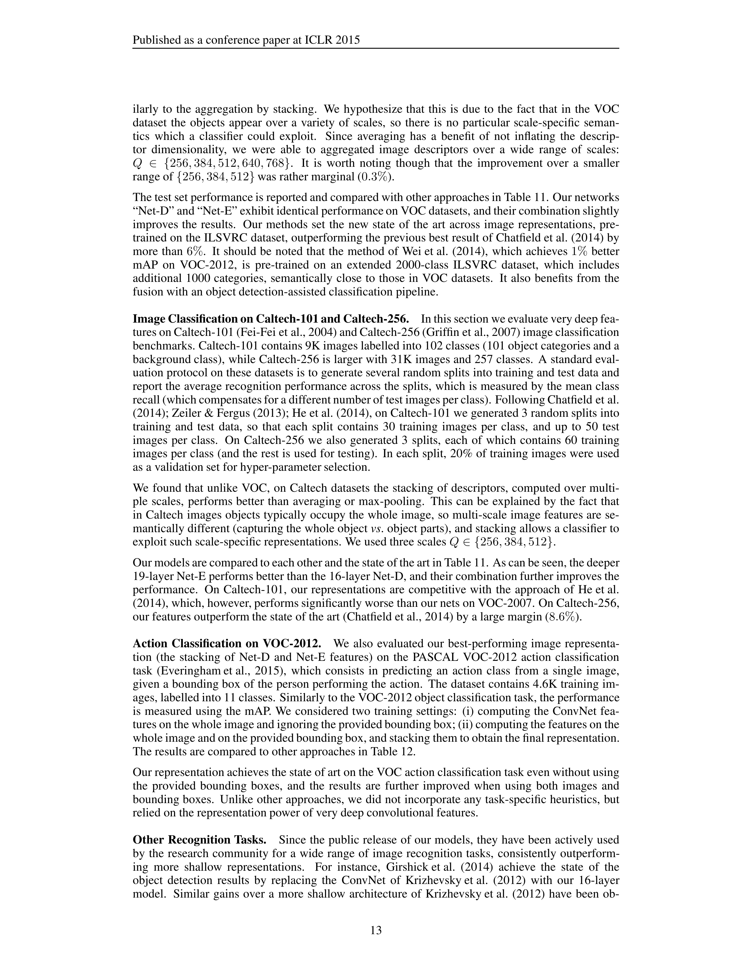
Table 11:
Comparison with the state of the art in image classification on VOC-2007, VOC-2012,
Caltech-101,
and
Caltech-256
.
Our
models are
denoted as
“VGG”.
Results
marked with
*
were
achieved using ConvNets pre-trained on the
extended
ILSVRC dataset (2000 classes).
Method
VOC-2007
VOC-2012
Caltech-101
Caltech-256
(mean AP)
(mean AP)
(mean class recall)
(mean class recall)
Zeiler & Fergus (Zeiler & Fergus, 2013)
-
79.0
86.5
±
0.5
74.2
±
0.3
Chatfield et al. (Chatfield et al., 2014)
82.4
83.2
88.4
±
0.6
77.6
±
0.1
He et al. (He et al., 2014)
82.4
-
93.4
±
0.5
-
Wei et al. (Wei et al., 2014)
81.5 (85.2
∗
)
81.7 (
90.3
∗
)
-
-
VGG Net-D (16 layers)
89.3
89.0
91.8
±
1.0
85.0
±
0.2
VGG Net-E (19 layers)
89.3
89.0
92.3
±
0.5
85.1
±
0.3
VGG Net-D & Net-E
89.7
89.3
92.7
±
0.5
86.2
±
0.3
Image Classification on VOC-2007 and VOC-2012.
We begin with the evaluation on the image
classification
task
of
PASCAL
VOC-2007
and
VOC-2012
benchmarks
(Everingham et al.,
2015).
These
datasets contain 10K and
22.5K images respectively, and each
image is
annotated with
one
or several labels, corresponding to 20 object categories.
The VOC organisers provide a pre-defined
split
into
training,
validation,
and
test
data
(the
test
data
for
VOC-2012
is
not
publicly
available;
instead, an official evaluation server is provided). Recognition performance is measured using mean
average precision (mAP) across classes.
Notably,
by
examining
the
performance
on
the
validation
sets
of
VOC-2007
and
VOC-2012,
we
found that aggregating image descriptors, computed at multiple scales, by averaging performs sim-
12
Published as a conference paper at ICLR 2015
ilarly
to
the
aggregation by
stacking.
We
hypothesize that
this
is
due
to
the
fact
that
in
the
VOC
dataset
the
objects
appear
over
a
variety
of
scales,
so
there
is
no
particular
scale-specific
seman-
tics
which
a
classifier
could
exploit.
Since
averaging
has
a
benefit
of
not
inflating
the
descrip-
tor
dimensionality,
we
were
able
to
aggregated
image
descriptors
over
a
wide
range
of
scales:
Q
∈{
256
,
384
,
512
,
640
,
768
}
.
It
is
worth
noting
though
that
the
improvement
over
a
smaller
range of
{
256
,
384
,
512
}
was rather marginal (
0
.
3%
).
The test set performance is reported and compared with other approaches in Table 11. Our networks
“Net-D” and “Net-E” exhibit identical performance on VOC datasets, and their combination slightly
improves the
results.
Our
methods
set
the
new
state
of
the
art
across
image
representations,
pre-
trained on the ILSVRC dataset, outperforming the previous best result of Chatfield et al. (2014) by
more
than
6%
.
It
should be
noted that
the
method of
Wei et al.
(2014),
which
achieves
1%
better
mAP
on
VOC-2012,
is
pre-trained
on
an
extended
2000-class
ILSVRC
dataset,
which
includes
additional
1000 categories,
semantically
close
to
those
in
VOC
datasets.
It
also
benefits
from
the
fusion with an object detection-assisted classification pipeline.
Image Classification on Caltech-101 and Caltech-256.
In this section we evaluate very deep fea-
tures on Caltech-101 (Fei-Fei et al., 2004) and Caltech-256 (Griffin et al., 2007) image classification
benchmarks. Caltech-101 contains 9K images labelled into 102 classes (101 object categories and a
background class), while Caltech-256 is larger with 31K images and 257 classes.
A standard eval-
uation protocol on these datasets is to generate several random splits into training and test data and
report the average recognition performance across the splits,
which is measured by the mean class
recall (which compensates for a different number of test images per class). Following Chatfield et al.
(2014); Zeiler & Fergus (2013); He et al. (2014), on Caltech-101 we generated 3 random splits into
training
and
test
data,
so
that
each
split
contains
30
training
images
per
class,
and
up
to
50
test
images
per
class.
On
Caltech-256
we
also
generated
3
splits,
each
of
which
contains
60
training
images per class (and the rest is used for testing).
In each split,
20% of training images were used
as a validation set for hyper-parameter selection.
We
found that
unlike
VOC,
on
Caltech
datasets
the
stacking
of
descriptors,
computed over multi-
ple
scales,
performs better
than
averaging or
max-pooling.
This
can
be
explained by
the
fact
that
in Caltech
images objects typically occupy the whole image,
so multi-scale image features are se-
mantically different (capturing the whole object
vs
. object parts), and stacking allows a classifier to
exploit such scale-specific representations. We used three scales
Q
∈{
256
,
384
,
512
}
.
Our models are compared to each other and the state of the art in Table 11. As can be seen, the deeper
19-layer Net-E performs better than the 16-layer Net-D, and their combination further improves the
performance.
On
Caltech-101,
our
representations
are
competitive
with
the
approach
of
He et al.
(2014), which, however, performs significantly worse than our nets on VOC-2007. On Caltech-256,
our features outperform the state of the art (Chatfield et al., 2014) by a large margin (
8
.
6%
).
Action
Classification
on
VOC-2012.
We
also
evaluated
our
best-performing image
representa-
tion
(the
stacking
of
Net-D
and
Net-E
features)
on
the
PASCAL
VOC-2012
action
classification
task
(Everingham et al.,
2015),
which
consists
in
predicting
an
action
class
from
a
single
image,
given a bounding box of the person performing the action.
The dataset contains 4.6K training im-
ages, labelled into 11 classes.
Similarly to the VOC-2012 object classification task, the performance
is
measured
using
the
mAP.
We
considered two
training settings:
(i)
computing the
ConvNet
fea-
tures on the whole image and ignoring the provided bounding box; (ii) computing the features on the
whole image and on the provided bounding box, and stacking them to obtain the final representation.
The results are compared to other approaches in Table 12.
Our representation achieves the state of art on the VOC action classification task even without using
the
provided
bounding
boxes,
and
the
results
are
further
improved
when
using
both
images
and
bounding boxes.
Unlike
other approaches, we
did not
incorporate any task-specific heuristics,
but
relied on the representation power of very deep convolutional features.
Other
Recognition Tasks.
Since
the
public release
of our models,
they
have been actively used
by
the
research
community for
a
wide
range
of
image
recognition tasks,
consistently
outperform-
ing
more
shallow
representations.
For
instance,
Girshick et al.
(2014)
achieve
the
state
of
the
object
detection
results
by
replacing
the
ConvNet
of
Krizhevsky et al.
(2012)
with
our
16-layer
model.
Similar
gains
over
a
more
shallow
architecture
of
Krizhevsky et al.
(2012)
have
been
ob-
13

Published as a conference paper at ICLR 2015
Table
12:
Comparison
with
the
state
of
the
art
in
single-image
action classification on
VOC-
2012
.
Our
models
are
denoted
as
“VGG”.
Results
marked
with
*
were
achieved using
ConvNets
pre-trained on the
extended
ILSVRC dataset (1512 classes).
Method
VOC-2012 (mean AP)
(Oquab et al., 2014)
70.2
∗
(Gkioxari et al., 2014)
73.6
(Hoai, 2014)
76.3
VGG Net-D & Net-E, image-only
79.2
VGG Net-D & Net-E, image and bounding box
84.0
served in
semantic
segmentation (Long et al.,
2014),
image
caption generation (Kiros et al.,
2014;
Karpathy & Fei-Fei, 2014), texture and material recognition (Cimpoi et al., 2014; Bell et al., 2014).
C
P
APER
R
EVISIONS
Here
we
present
the
list
of
major
paper revisions,
outlining the
substantial
changes for the
conve-
nience of the reader.
v1
Initial version. Presents the experiments carried out before the ILSVRC submission.
v2
Adds post-submission ILSVRC experiments with training set augmentation using scale jittering,
which improves the performance.
v3
Adds generalisation experiments (Appendix B) on PASCAL VOC and Caltech image classifica-
tion datasets.
The models used for these experiments are publicly available.
v4
The paper is converted to ICLR-2015 submission format.
Also adds experiments with multiple
crops for classification.
v6
Camera-ready ICLR-2015 conference paper.
Adds a comparison of the net B with a shallow net
and the results on PASCAL VOC action classification benchmark.
14