You Only Look Once:
Unified, Real-Time Object Detection
Joseph Redmon
∗
, Santosh Divvala
∗†
, Ross Girshick
¶
, Ali Farhadi
∗†
University of Washington
∗
, Allen Institute for AI
†
, Facebook AI Research
¶
http://pjreddie.com/yolo/
Abstract
We
present
YOLO,
a
new
approach
to
object
detection.
Prior work on object detection repurposes classifiers to per-
form detection.
Instead, we frame object detection as a re-
gression problem to spatially separated bounding boxes and
associated class probabilities.
A single neural network pre-
dicts
bounding
boxes
and
class
probabilities
directly
from
full
images
in
one
evaluation.
Since
the
whole
detection
pipeline is a single network, it can be optimized end-to-end
directly on detection performance.
Our
unified
architecture
is
extremely
fast.
Our
base
YOLO
model
processes
images
in
real-time
at
45
frames
per second.
A smaller version of the network,
Fast YOLO,
processes
an
astounding
155
frames
per
second
while
still
achieving
double
the
mAP
of
other
real-time
detec-
tors. Compared to state-of-the-art detection systems, YOLO
makes
more
localization
errors
but
is
less
likely
to
predict
false
positives
on
background.
Finally,
YOLO
learns
very
general representations of objects.
It outperforms other de-
tection methods,
including DPM and R-CNN, when gener-
alizing from natural images to other domains like artwork.
1. Introduction
Humans glance at an image and instantly know what ob-
jects
are
in
the
image,
where
they
are,
and
how
they
inter-
act.
The
human
visual
system
is
fast
and
accurate,
allow-
ing us to perform complex tasks like driving with little con-
scious
thought.
Fast,
accurate
algorithms
for
object
detec-
tion
would
allow
computers
to
drive
cars
without
special-
ized
sensors,
enable
assistive
devices
to
convey
real-time
scene information to human users, and unlock the potential
for general purpose, responsive robotic systems.
Current
detection
systems
repurpose
classifiers
to
per-
form
detection.
To
detect
an
object,
these
systems
take
a
classifier for that object and evaluate it at various locations
and
scales
in
a
test
image.
Systems
like
deformable
parts
models
(DPM)
use
a
sliding
window
approach
where
the
classifier
is
run
at
evenly
spaced
locations
over
the
entire
image [
10
].
More recent approaches like R-CNN use region proposal
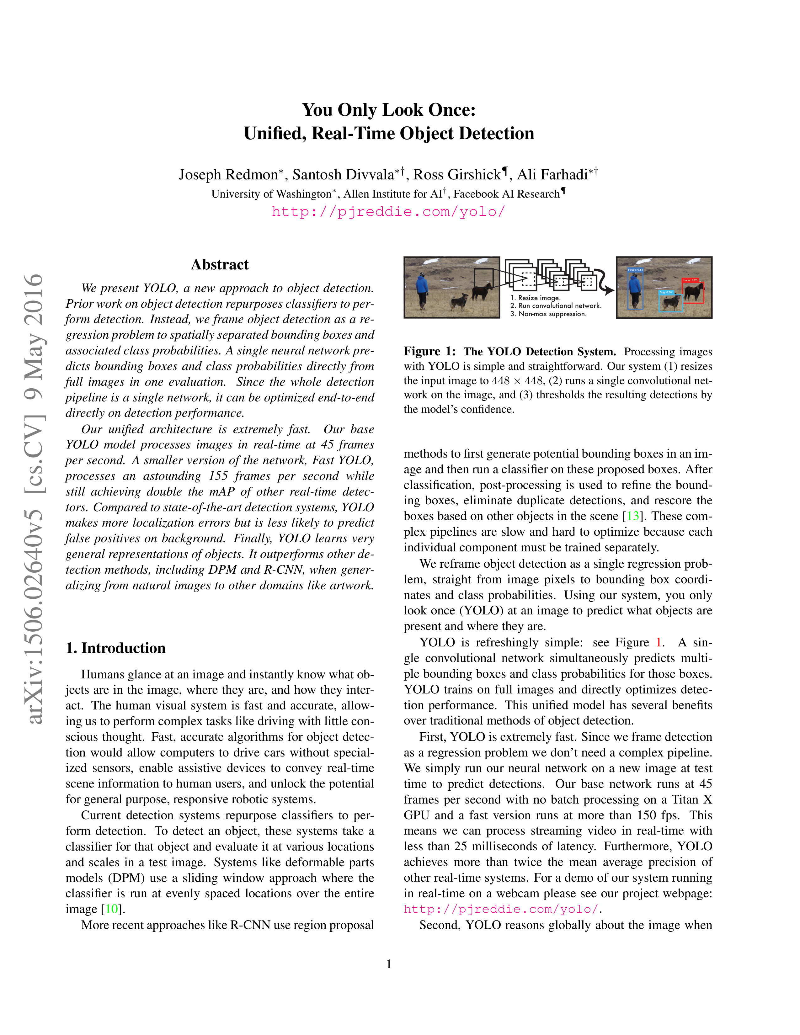
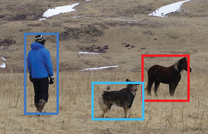
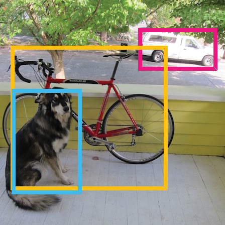
1. Resize image.
2. Run convolutional network.
3. Non-max suppression.
Dog: 0.30
Person: 0.64
Horse: 0.28
Figure
1:
The
YOLO
Detection
System.
Processing
images
with YOLO is simple and straightforward.
Our system (1) resizes
the input image to
448
×
448
, (2) runs a single convolutional net-
work on the image, and (3) thresholds the resulting detections by
the model’s confidence.
methods to first generate potential bounding boxes in an im-
age and then run a classifier on these proposed boxes.
After
classification,
post-processing
is
used
to
refine
the
bound-
ing
boxes,
eliminate
duplicate
detections,
and
rescore
the
boxes based on other objects in the scene [
13
].
These com-
plex
pipelines
are
slow
and
hard
to
optimize
because
each
individual component must be trained separately.
We reframe object detection as a single regression prob-
lem,
straight
from
image
pixels
to
bounding
box
coordi-
nates
and
class
probabilities.
Using
our
system,
you
only
look once (YOLO) at an image to predict what objects are
present and where they are.
YOLO
is
refreshingly
simple:
see
Figure
1
.
A
sin-
gle
convolutional
network
simultaneously
predicts
multi-
ple bounding boxes and class probabilities for those boxes.
YOLO
trains
on
full
images
and
directly
optimizes
detec-
tion
performance.
This
unified
model
has
several
benefits
over traditional methods of object detection.
First, YOLO is extremely fast.
Since we frame detection
as a regression problem we don’t need a complex pipeline.
We
simply
run
our
neural
network
on
a
new
image
at
test
time
to
predict
detections.
Our
base
network
runs
at
45
frames
per
second
with
no
batch
processing
on
a
Titan
X
GPU
and
a
fast
version
runs
at
more
than
150
fps.
This
means
we
can
process
streaming
video
in
real-time
with
less
than
25
milliseconds
of
latency.
Furthermore,
YOLO
achieves
more
than
twice
the
mean
average
precision
of
other real-time systems.
For a demo of our system running
in
real-time
on
a
webcam
please
see
our
project
webpage:
http://pjreddie.com/yolo/
.
Second,
YOLO
reasons
globally
about
the
image
when
1
arXiv:1506.02640v5 [cs.CV] 9 May 2016
making
predictions.
Unlike
sliding
window
and
region
proposal-based
techniques,
YOLO
sees
the
entire
image
during training and test time so it implicitly encodes contex-
tual
information
about
classes
as
well
as
their
appearance.
Fast
R-CNN,
a
top
detection
method
[
14
],
mistakes
back-
ground patches in an image for objects because it can’t see
the larger context.
YOLO makes less than half the number
of background errors compared to Fast R-CNN.
Third, YOLO learns generalizable representations of ob-
jects.
When
trained
on
natural
images
and
tested
on
art-
work, YOLO outperforms top detection methods like DPM
and R-CNN by a wide margin.
Since YOLO is highly gen-
eralizable
it
is
less
likely
to
break
down
when
applied
to
new domains or unexpected inputs.
YOLO still lags behind state-of-the-art detection systems
in
accuracy.
While
it
can
quickly
identify
objects
in
im-
ages
it
struggles
to
precisely
localize
some
objects,
espe-
cially small ones.
We examine these tradeoffs further in our
experiments.
All
of
our
training
and
testing
code
is
open
source.
A
variety of pretrained models are also available to download.
2. Unified Detection
We
unify
the
separate
components
of
object
detection
into
a
single
neural
network.
Our
network
uses
features
from the entire image to predict each bounding box.
It also
predicts
all
bounding
boxes
across
all
classes
for
an
im-
age simultaneously.
This means our network reasons glob-
ally
about
the
full
image
and
all
the
objects
in
the
image.
The
YOLO
design
enables
end-to-end
training
and
real-
time speeds while maintaining high average precision.
Our system divides the input image into an
S
×
S
grid.
If the center of an object falls into a grid cell, that grid cell
is responsible for detecting that object.
Each grid cell predicts
B
bounding boxes and confidence
scores for those boxes.
These confidence scores reflect how
confident
the
model
is
that
the
box
contains
an
object
and
also
how
accurate
it
thinks
the
box
is
that
it
predicts.
For-
mally we define confidence as
Pr(
Object
)
∗
IOU
truth
pred
.
If no
object
exists
in
that
cell,
the
confidence
scores
should
be
zero.
Otherwise we want the confidence score to equal the
intersection
over
union
(IOU)
between
the
predicted
box
and the ground truth.
Each bounding box consists of 5 predictions:
x
,
y
,
w
,
h
,
and confidence.
The
(
x, y
)
coordinates represent the center
of the box relative to the bounds of the grid cell.
The width
and height are predicted relative to the whole image. Finally
the
confidence
prediction
represents
the
IOU
between
the
predicted box and any ground truth box.
Each
grid
cell
also
predicts
C
conditional
class
proba-
bilities,
Pr(
Class
i
|
Object
)
.
These
probabilities
are
condi-
tioned on the grid cell containing an object. We only predict
one set of class probabilities per grid cell, regardless of the
number of boxes
B
.
At test time we multiply the conditional class probabili-
ties and the individual box confidence predictions,
Pr(
Class
i
|
Object
)
∗
Pr(
Object
)
∗
IOU
truth
pred
=
Pr(
Class
i
)
∗
IOUtruth
pred
(1)
which
gives
us
class-specific
confidence
scores
for
each
box.
These scores encode both the probability of that class
appearing in the box and how well the predicted box fits the
object.
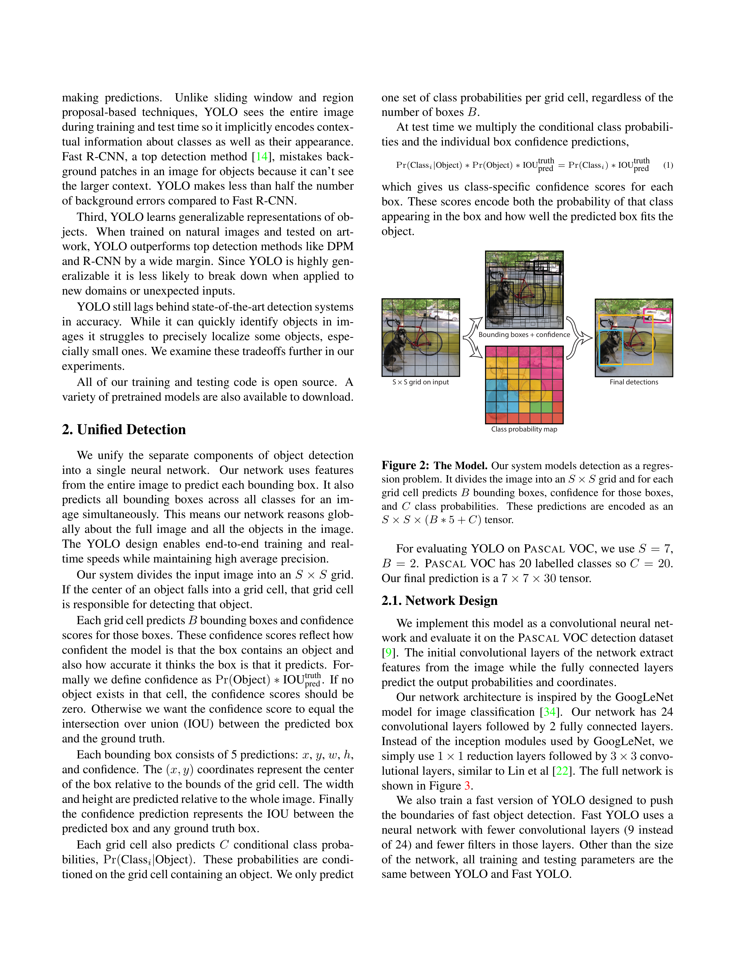
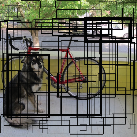
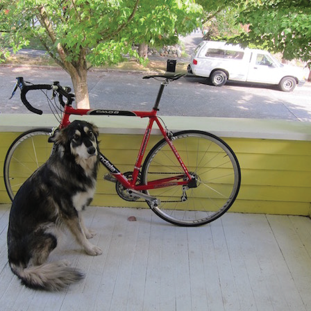
S × S grid on input
Bounding boxes + confidence
Class probability map
Final detections
Figure 2:
The Model.
Our system models detection as a regres-
sion problem.
It divides the image into an
S
×
S
grid and for each
grid
cell
predicts
B
bounding
boxes,
confidence
for
those
boxes,
and
C
class
probabilities.
These
predictions
are
encoded
as
an
S
×
S
×
(
B
∗
5 +
C
)
tensor.
For evaluating YOLO on
P
ASCAL
VOC, we use
S
=
7
,
B
=
2
.
P
ASCAL
VOC has 20 labelled classes so
C
=
20
.
Our final prediction is a
7
×
7
×
30
tensor.
2.1. Network Design
We implement this model as a convolutional neural net-
work and evaluate it on the P
ASCAL
VOC detection dataset
[
9
].
The initial convolutional layers of the network extract
features
from
the
image
while
the
fully
connected
layers
predict the output probabilities and coordinates.
Our
network
architecture
is
inspired
by
the
GoogLeNet
model
for
image
classification
[
34
].
Our
network
has
24
convolutional
layers
followed
by
2
fully
connected
layers.
Instead
of
the
inception
modules
used
by
GoogLeNet,
we
simply use
1
×
1
reduction layers followed by
3
×
3
convo-
lutional layers, similar to Lin et al [
22
].
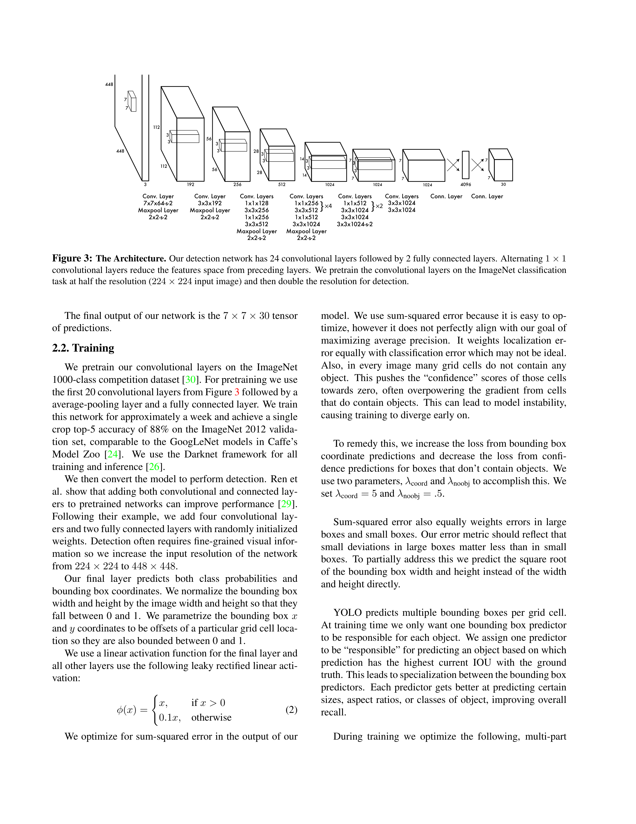
The full network is
shown in Figure
3
.
We
also
train
a
fast
version
of
YOLO
designed
to
push
the
boundaries
of
fast
object
detection.
Fast
YOLO
uses
a
neural
network
with
fewer
convolutional
layers
(9
instead
of 24) and fewer filters in those layers.
Other than the size
of
the
network,
all
training
and
testing
parameters
are
the
same between YOLO and Fast YOLO.
448
448
3
7
7
Conv. Layer
7x7x64-s-2
Maxpool Layer
2x2-s-2
3
3
112
112
192
3
3
56
56
256
Conn. Layer
4096
Conn. Layer
Conv. Layer
3x3x192
Maxpool Layer
2x2-s-2
Conv. Layers
1x1x128
3x3x256
1x1x256
3x3x512
Maxpool Layer
2x2-s-2
3
3
28
28
512
Conv. Layers
1x1x256
3x3x512
1x1x512
3x3x1024
Maxpool Layer
2x2-s-2
3
3
14
14
1024
Conv. Layers
1x1x512
3x3x1024
3x3x1024
3x3x1024-s-2
3
3
7
7
1024
7
7
1024
7
7
30
}
×4
}
×2
Conv. Layers
3x3x1024
3x3x1024
Figure 3:
The Architecture.
Our detection network has 24 convolutional layers followed by 2 fully connected layers.
Alternating
1
×
1
convolutional layers reduce the features space from preceding layers.
We pretrain the convolutional layers on the ImageNet classification
task at half the resolution (
224
×
224
input image) and then double the resolution for detection.
The final output of our network is the
7
×
7
×
30
tensor
of predictions.
2.2. Training
We
pretrain
our
convolutional
layers
on
the
ImageNet
1000-class competition dataset [
30
].
For pretraining we use
the first 20 convolutional layers from Figure
3
followed by a
average-pooling layer and a fully connected layer.
We train
this network for approximately a week and achieve a single
crop
top-5 accuracy
of
88%
on
the
ImageNet
2012
valida-
tion
set,
comparable
to
the
GoogLeNet
models
in
Caffe’s
Model
Zoo
[
24
].
We
use
the
Darknet
framework
for
all
training and inference [
26
].
We then convert the model to perform detection.
Ren et
al.
show that adding both convolutional and connected lay-
ers
to
pretrained
networks
can
improve
performance
[
29
].
Following
their
example,
we
add
four
convolutional
lay-
ers and two fully connected layers with randomly initialized
weights.
Detection often requires fine-grained visual infor-
mation
so
we
increase
the
input
resolution
of
the
network
from
224
×
224
to
448
×
448
.
Our
final
layer
predicts
both
class
probabilities
and
bounding box coordinates.
We normalize the bounding box
width and height by the image width and height so that they
fall
between
0
and
1.
We
parametrize
the
bounding
box
x
and
y
coordinates to be offsets of a particular grid cell loca-
tion so they are also bounded between 0 and 1.
We use a linear activation function for the final layer and
all other layers use the following leaky rectified linear acti-
vation:
φ
(
x
) =
(
x,
if
x >
0
0
.
1
x,
otherwise
(2)
We
optimize
for
sum-squared
error
in
the
output
of
our
model.
We use sum-squared error because it is easy to op-
timize, however it does not perfectly align with our goal of
maximizing
average
precision.
It
weights
localization
er-
ror equally with classification error which may not be ideal.
Also,
in
every
image
many
grid
cells
do
not
contain
any
object.
This
pushes
the
“confidence”
scores
of
those
cells
towards
zero,
often
overpowering
the
gradient
from
cells
that
do
contain
objects.
This
can
lead
to
model
instability,
causing training to diverge early on.
To remedy this, we increase the loss from bounding box
coordinate
predictions
and
decrease
the
loss
from
confi-
dence predictions for boxes that don’t contain objects.
We
use two parameters,
λ
coord
and
λ
noobj
to accomplish this. We
set
λ
coord
= 5
and
λ
noobj
=
.
5
.
Sum-squared
error
also
equally
weights
errors
in
large
boxes and small boxes.
Our error metric should reflect that
small
deviations
in
large
boxes
matter
less
than
in
small
boxes.
To
partially
address
this
we
predict
the
square
root
of the bounding box width and height instead of the width
and height directly.
YOLO
predicts
multiple
bounding
boxes
per
grid
cell.
At training time we only want one bounding box predictor
to
be
responsible
for
each
object.
We
assign
one
predictor
to be “responsible” for predicting an object based on which
prediction
has
the
highest
current
IOU
with
the
ground
truth. This leads to specialization between the bounding box
predictors.
Each
predictor
gets
better
at
predicting
certain
sizes,
aspect
ratios,
or
classes
of
object,
improving
overall
recall.
During
training
we
optimize
the
following,
multi-part
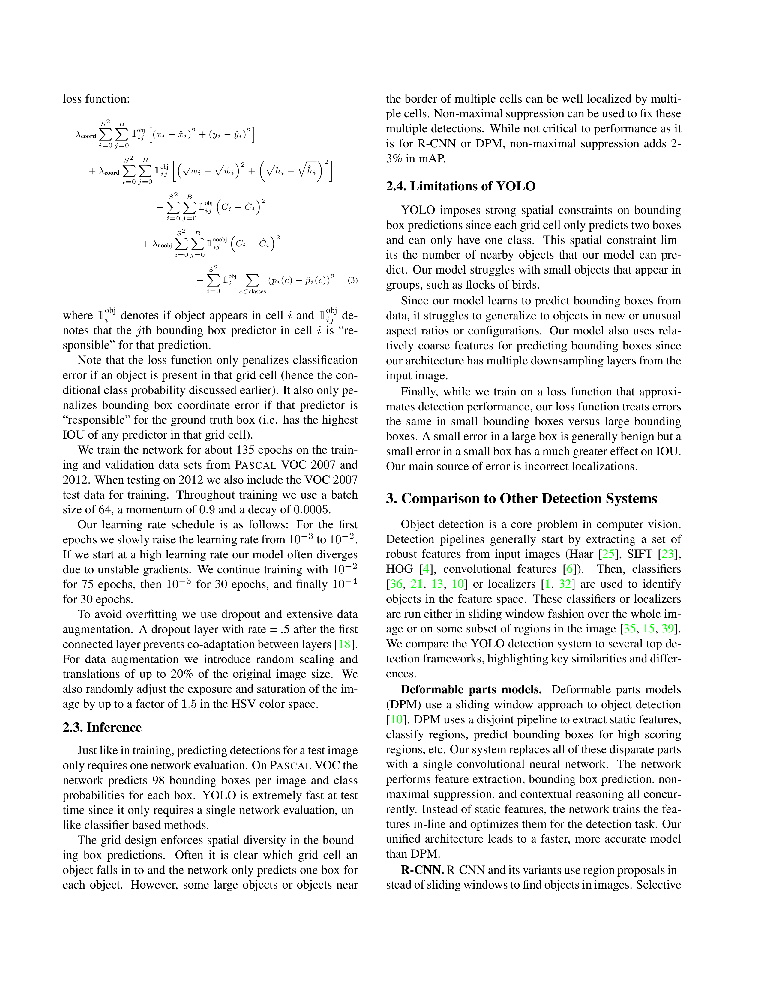
loss function:
λ
coord
S
2
X
i
=0
B
X
j
=0
1
obj
ij
h
(
x
i
−
ˆ
x
i
)
2
+ (
y
i
−
ˆ
y
i
)
2
i
+
λ
coord
S
2
X
i
=0
B
X
j
=0
1
obj
ij
√
w
i
−
p
ˆ
w
i
2
+
p
h
i
−
q
ˆ
h
i
2
+
S
2
X
i
=0
B
X
j
=0
1
obj
ij
C
i
−
ˆ
C
i
2
+
λ
noobj
S
2
X
i
=0
B
X
j
=0
1
noobj
ij
C
i
−
ˆ
C
i
2
+
S
2
X
i
=0
1
obj
i
X
c
∈
classes
(
p
i
(
c
)
−
ˆ
p
i
(
c
))
2
(3)
where
1
obj
i
denotes
if
object
appears
in
cell
i
and
1
obj
ij
de-
notes
that
the
j
th
bounding
box
predictor
in
cell
i
is
“re-
sponsible” for that prediction.
Note
that
the
loss
function
only
penalizes
classification
error if an object is present in that grid cell (hence the con-
ditional class probability discussed earlier).
It also only pe-
nalizes
bounding
box
coordinate
error
if
that
predictor
is
“responsible” for the ground truth box (i.e.
has the highest
IOU of any predictor in that grid cell).
We train the network for about 135 epochs on the train-
ing
and
validation
data
sets
from
P
ASCAL
VOC
2007
and
2012.
When testing on 2012 we also include the VOC 2007
test
data
for
training.
Throughout
training
we
use
a
batch
size of 64, a momentum of
0
.
9
and a decay of
0
.
0005
.
Our
learning
rate
schedule
is
as
follows:
For
the
first
epochs we slowly raise the learning rate from
10
−
3
to
10
−
2
.
If we start at a high learning rate our model often diverges
due to unstable gradients.
We continue training with
10
−
2
for
75
epochs,
then
10
−
3
for
30
epochs,
and
finally
10
−
4
for 30 epochs.
To
avoid
overfitting
we
use
dropout
and
extensive
data
augmentation.
A dropout layer with rate = .5 after the first
connected layer prevents co-adaptation between layers [
18
].
For
data
augmentation
we
introduce
random
scaling
and
translations
of
up
to
20%
of
the
original
image
size.
We
also randomly adjust the exposure and saturation of the im-
age by up to a factor of
1
.
5
in the HSV color space.
2.3. Inference
Just like in training, predicting detections for a test image
only requires one network evaluation. On P
ASCAL
VOC the
network
predicts
98
bounding
boxes
per
image
and
class
probabilities
for
each
box.
YOLO
is
extremely
fast
at
test
time since it only requires a single network evaluation, un-
like classifier-based methods.
The
grid
design
enforces
spatial
diversity
in
the
bound-
ing
box
predictions.
Often
it
is
clear
which
grid
cell
an
object falls in to and the network only predicts one box for
each
object.
However,
some
large
objects
or
objects
near
the border of multiple cells can be well localized by multi-
ple cells.
Non-maximal suppression can be used to fix these
multiple detections.
While not critical to performance as it
is
for
R-CNN
or
DPM,
non-maximal
suppression
adds
2-
3% in mAP.
2.4. Limitations of YOLO
YOLO
imposes
strong
spatial
constraints
on
bounding
box predictions since each grid cell only predicts two boxes
and
can
only
have
one
class.
This
spatial
constraint
lim-
its
the
number
of
nearby
objects
that
our
model
can
pre-
dict.
Our model struggles with small objects that appear in
groups, such as flocks of birds.
Since
our
model
learns
to
predict
bounding
boxes
from
data, it struggles to generalize to objects in new or unusual
aspect
ratios
or
configurations.
Our
model
also
uses
rela-
tively
coarse
features
for
predicting
bounding
boxes
since
our architecture has multiple downsampling layers from the
input image.
Finally,
while
we
train
on
a
loss
function
that
approxi-
mates detection performance, our loss function treats errors
the
same
in
small
bounding
boxes
versus
large
bounding
boxes.
A small error in a large box is generally benign but a
small error in a small box has a much greater effect on IOU.
Our main source of error is incorrect localizations.
3. Comparison to Other Detection Systems
Object
detection
is
a
core
problem
in
computer
vision.
Detection
pipelines
generally
start
by
extracting
a
set
of
robust
features
from
input
images
(Haar
[
25
],
SIFT
[
23
],
HOG
[
4
],
convolutional
features
[
6
]).
Then,
classifiers
[
36
,
21
,
13
,
10
]
or
localizers
[
1
,
32
]
are
used
to
identify
objects
in
the
feature
space.
These
classifiers
or
localizers
are run either in sliding window fashion over the whole im-
age or on some subset of regions in the image [
35
,
15
,
39
].
We compare the YOLO detection system to several top de-
tection frameworks, highlighting key similarities and differ-
ences.
Deformable
parts
models.
Deformable
parts
models
(DPM)
use
a
sliding
window
approach
to
object
detection
[
10
].
DPM uses a disjoint pipeline to extract static features,
classify
regions,
predict
bounding
boxes
for
high
scoring
regions, etc. Our system replaces all of these disparate parts
with
a
single
convolutional
neural
network.
The
network
performs feature extraction, bounding box prediction, non-
maximal suppression, and contextual reasoning all concur-
rently.
Instead of static features, the network trains the fea-
tures in-line and optimizes them for the detection task.
Our
unified
architecture
leads
to
a
faster,
more
accurate
model
than DPM.
R-CNN.
R-CNN and its variants use region proposals in-
stead of sliding windows to find objects in images. Selective
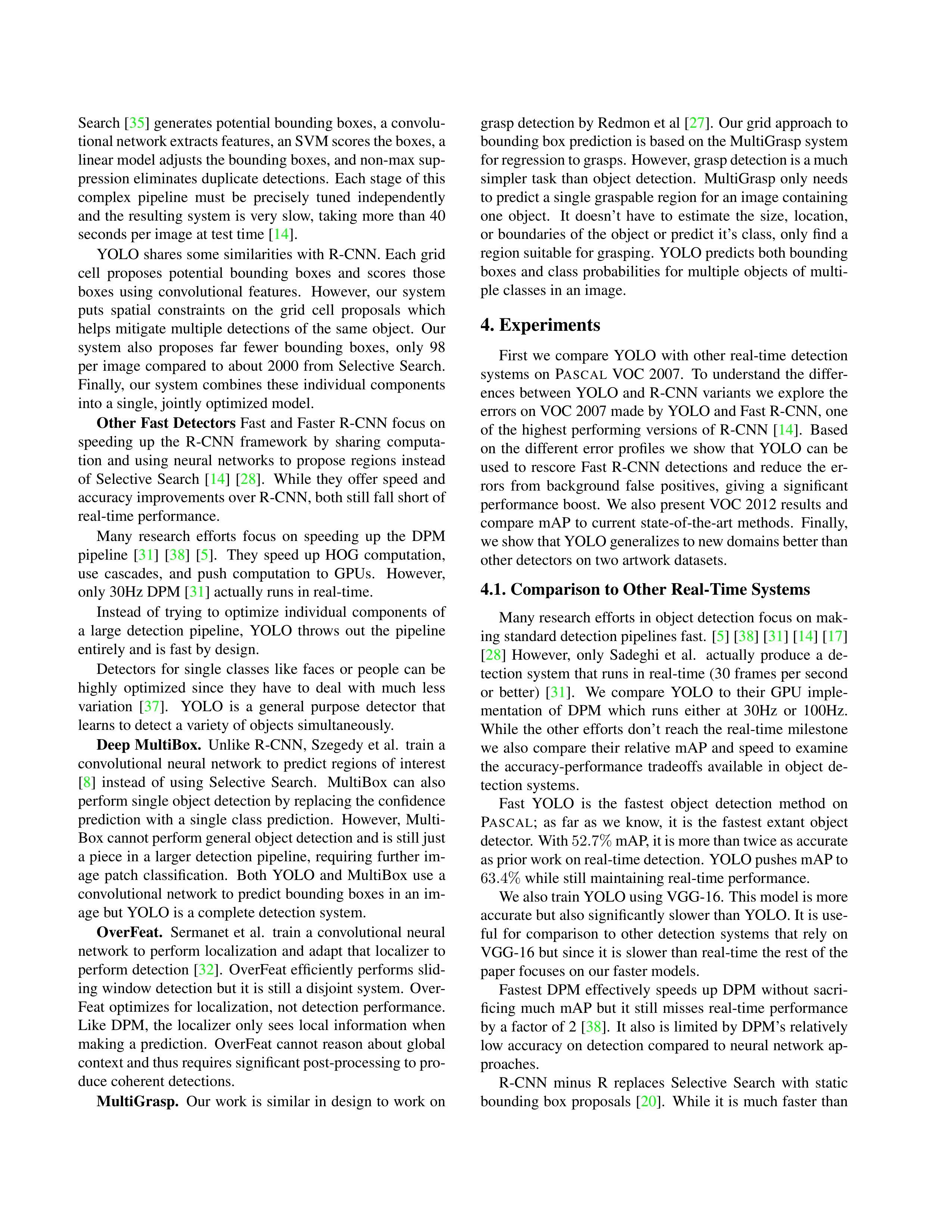
Search [
35
] generates potential bounding boxes, a convolu-
tional network extracts features, an SVM scores the boxes, a
linear model adjusts the bounding boxes, and non-max sup-
pression eliminates duplicate detections.
Each stage of this
complex
pipeline
must
be
precisely
tuned
independently
and the resulting
system
is
very
slow,
taking
more
than
40
seconds per image at test time [
14
].
YOLO shares some similarities with R-CNN. Each grid
cell
proposes
potential
bounding
boxes
and
scores
those
boxes
using
convolutional
features.
However,
our
system
puts
spatial
constraints
on
the
grid
cell
proposals
which
helps
mitigate
multiple
detections
of
the
same
object.
Our
system
also
proposes
far
fewer
bounding
boxes,
only
98
per
image
compared
to
about
2000
from
Selective
Search.
Finally,
our
system
combines
these
individual
components
into a single, jointly optimized model.
Other Fast Detectors
Fast and Faster R-CNN focus on
speeding
up
the
R-CNN
framework
by
sharing
computa-
tion
and
using
neural
networks
to
propose
regions
instead
of
Selective
Search
[
14
]
[
28
].
While
they
offer
speed
and
accuracy improvements over R-CNN, both still fall short of
real-time performance.
Many
research
efforts
focus
on
speeding
up
the
DPM
pipeline
[
31
]
[
38
]
[
5
].
They
speed
up
HOG
computation,
use
cascades,
and
push
computation
to
GPUs.
However,
only 30Hz DPM [
31
] actually runs in real-time.
Instead
of
trying
to
optimize
individual
components
of
a
large
detection
pipeline,
YOLO
throws
out
the
pipeline
entirely and is fast by design.
Detectors
for
single
classes
like
faces
or
people
can
be
highly
optimized
since
they
have
to
deal
with
much
less
variation
[
37
].
YOLO
is
a
general
purpose
detector
that
learns to detect a variety of objects simultaneously.
Deep MultiBox.
Unlike R-CNN, Szegedy et al.
train a
convolutional
neural
network
to
predict
regions
of
interest
[
8
]
instead
of
using
Selective
Search.
MultiBox
can
also
perform single object detection by replacing the confidence
prediction
with
a
single
class
prediction.
However,
Multi-
Box cannot perform general object detection and is still just
a
piece in a larger detection
pipeline,
requiring
further im-
age
patch
classification.
Both
YOLO
and
MultiBox
use
a
convolutional network to predict bounding boxes in an im-
age but YOLO is a complete detection system.
OverFeat.
Sermanet
et
al.
train
a
convolutional
neural
network
to
perform
localization
and
adapt
that
localizer
to
perform detection [
32
].
OverFeat efficiently performs slid-
ing window detection but it is still a disjoint system.
Over-
Feat optimizes for localization,
not detection performance.
Like
DPM,
the
localizer
only
sees
local
information
when
making a prediction.
OverFeat
cannot
reason
about global
context and thus requires significant post-processing to pro-
duce coherent detections.
MultiGrasp.
Our
work
is
similar
in
design
to
work
on
grasp detection by Redmon et al [
27
].
Our grid approach to
bounding box prediction is based on the MultiGrasp system
for regression to grasps. However, grasp detection is a much
simpler
task
than
object
detection.
MultiGrasp
only
needs
to predict a single graspable region for an image containing
one
object.
It
doesn’t
have
to
estimate
the
size,
location,
or boundaries of the object or predict it’s class, only find a
region suitable for grasping.
YOLO predicts both bounding
boxes and class probabilities for multiple objects of multi-
ple classes in an image.
4. Experiments
First
we
compare
YOLO
with
other
real-time
detection
systems
on
P
ASCAL
VOC
2007.
To
understand
the
differ-
ences between YOLO and R-CNN variants we explore the
errors on VOC 2007 made by YOLO and Fast R-CNN, one
of
the
highest
performing
versions
of
R-CNN
[
14
].
Based
on
the
different
error
profiles
we
show
that
YOLO
can
be
used
to
rescore
Fast
R-CNN
detections
and
reduce
the
er-
rors
from
background
false
positives,
giving
a
significant
performance boost.
We also present VOC 2012 results and
compare
mAP
to
current
state-of-the-art
methods.
Finally,
we show that YOLO generalizes to new domains better than
other detectors on two artwork datasets.
4.1. Comparison to Other Real-Time Systems
Many research efforts in object detection focus on mak-
ing standard detection pipelines fast.
[
5
] [
38
] [
31
] [
14
] [
17
]
[
28
]
However,
only
Sadeghi
et
al.
actually
produce
a
de-
tection system that runs in real-time (30 frames per second
or
better)
[
31
].
We
compare
YOLO
to
their
GPU
imple-
mentation
of
DPM
which
runs
either
at
30Hz
or
100Hz.
While
the
other
efforts
don’t
reach
the
real-time
milestone
we
also
compare
their
relative
mAP
and
speed
to
examine
the
accuracy-performance
tradeoffs
available
in
object
de-
tection systems.
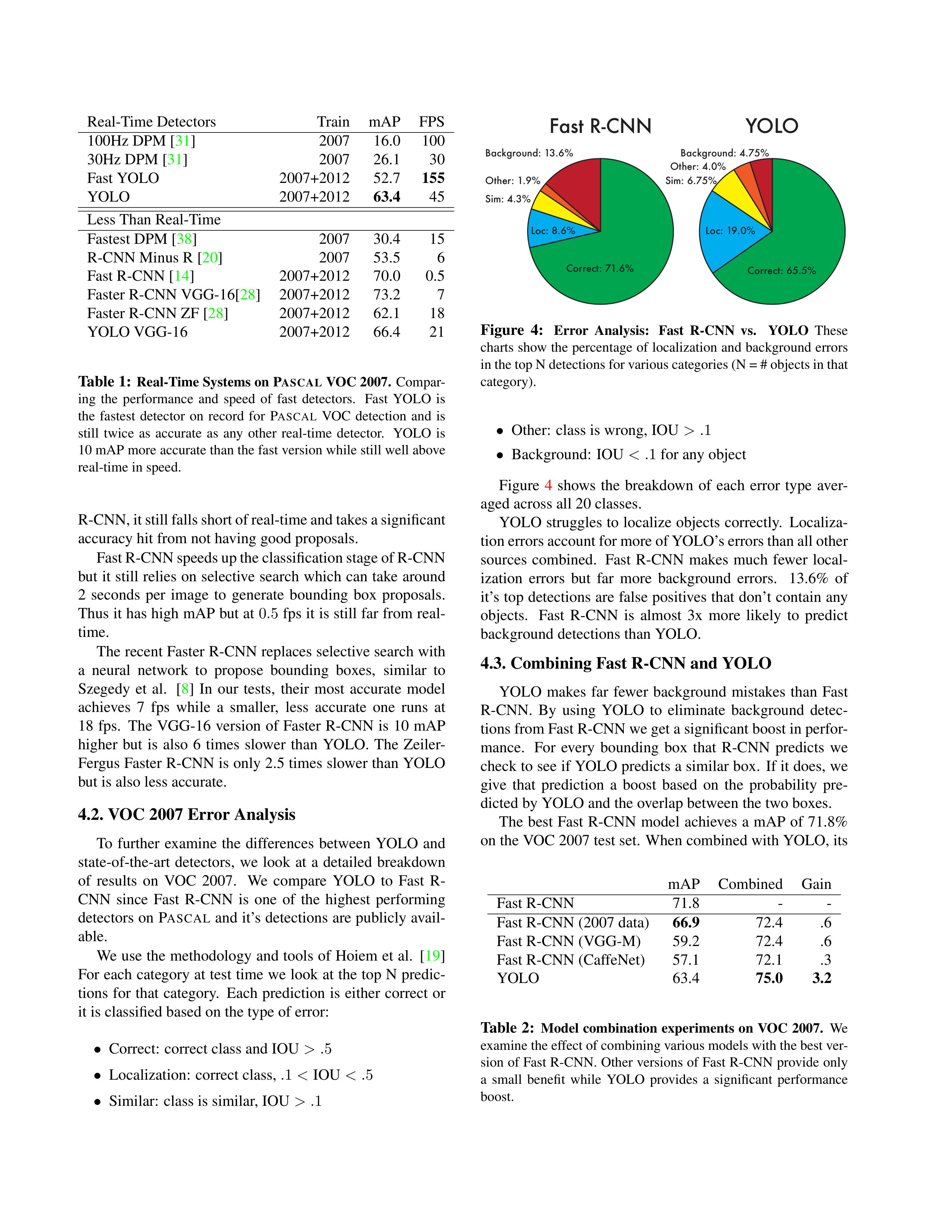
Fast
YOLO
is
the
fastest
object
detection
method
on
P
ASCAL
;
as
far
as
we
know,
it
is
the
fastest
extant
object
detector. With
52
.
7%
mAP, it is more than twice as accurate
as prior work on real-time detection. YOLO pushes mAP to
63
.
4%
while still maintaining real-time performance.
We also train YOLO using VGG-16.
This model is more
accurate but also significantly slower than YOLO. It is use-
ful
for
comparison
to
other
detection
systems
that
rely
on
VGG-16 but since it is slower than real-time the rest of the
paper focuses on our faster models.
Fastest
DPM
effectively
speeds
up
DPM
without
sacri-
ficing
much
mAP
but
it
still
misses
real-time
performance
by a factor of 2 [
38
].
It also is limited by DPM’s relatively
low accuracy on detection compared to neural network ap-
proaches.
R-CNN
minus
R
replaces
Selective
Search
with
static
bounding box
proposals [
20
].
While it is
much faster
than
Real-Time Detectors
Train
mAP
FPS
100Hz DPM [
31
]
2007
16.0
100
30Hz DPM [
31
]
2007
26.1
30
Fast YOLO
2007+2012
52.7
155
YOLO
2007+2012
63.4
45
Less Than Real-Time
Fastest DPM [
38
]
2007
30.4
15
R-CNN Minus R [
20
]
2007
53.5
6
Fast R-CNN [
14
]
2007+2012
70.0
0.5
Faster R-CNN VGG-16[
28
]
2007+2012
73.2
7
Faster R-CNN ZF [
28
]
2007+2012
62.1
18
YOLO VGG-16
2007+2012
66.4
21
Table 1:
Real-Time Systems on P
ASCAL
VOC 2007.
Compar-
ing
the
performance
and
speed
of
fast
detectors.
Fast
YOLO
is
the
fastest
detector
on
record
for
P
ASCAL
VOC
detection
and
is
still
twice
as
accurate
as
any
other
real-time
detector.
YOLO
is
10 mAP more accurate than the fast version while still well above
real-time in speed.
R-CNN, it still falls short of real-time and takes a significant
accuracy hit from not having good proposals.
Fast R-CNN speeds up the classification stage of R-CNN
but it still relies on selective search which can take around
2
seconds
per
image
to
generate
bounding
box
proposals.
Thus it has high mAP but at
0
.
5
fps it is still far from real-
time.
The recent Faster R-CNN replaces selective search with
a
neural
network
to
propose
bounding
boxes,
similar
to
Szegedy
et
al.
[
8
]
In
our
tests,
their
most
accurate
model
achieves
7
fps
while
a
smaller,
less
accurate
one
runs
at
18
fps.
The
VGG-16
version
of
Faster
R-CNN
is
10
mAP
higher
but
is
also
6
times
slower
than
YOLO.
The
Zeiler-
Fergus Faster R-CNN is only 2.5 times slower than YOLO
but is also less accurate.
4.2. VOC 2007 Error Analysis
To
further
examine
the
differences
between
YOLO
and
state-of-the-art
detectors,
we
look
at
a
detailed
breakdown
of
results
on
VOC
2007.
We
compare
YOLO
to
Fast
R-
CNN
since
Fast
R-CNN
is
one
of
the
highest
performing
detectors on
P
ASCAL
and it’s detections are publicly avail-
able.
We use the methodology and tools of Hoiem et al.
[
19
]
For each category at test time we look at the top N predic-
tions
for
that
category.
Each
prediction
is
either
correct
or
it is classified based on the type of error:
•
Correct:
correct class and IOU
> .
5
•
Localization:
correct class,
.
1
<
IOU
< .
5
•
Similar:
class is similar, IOU
> .
1
Correct: 71.6%
Correct: 65.5%
Loc: 8.6%
Sim: 4.3%
Other: 1.9%
Background: 13.6%
Loc: 19.0%
Sim: 6.75%
Other: 4.0%
Background: 4.75%
Fast R-CNN
YOLO
Figure
4:
Error
Analysis:
Fast
R-CNN
vs.
YOLO
These
charts show the percentage of localization and background errors
in the top N detections for various categories (N = # objects in that
category).
•
Other:
class is wrong, IOU
> .
1
•
Background:
IOU
< .
1
for any object
Figure
4
shows
the
breakdown
of
each
error
type
aver-
aged across all 20 classes.
YOLO struggles to localize objects correctly.
Localiza-
tion errors account for more of YOLO’s errors than all other
sources
combined.
Fast
R-CNN
makes
much
fewer
local-
ization
errors
but
far
more
background
errors.
13.6%
of
it’s top detections are false positives that don’t contain any
objects.
Fast
R-CNN
is
almost
3x
more
likely
to
predict
background detections than YOLO.
4.3. Combining Fast R-CNN and YOLO
YOLO
makes
far
fewer
background
mistakes
than
Fast
R-CNN.
By
using
YOLO
to
eliminate
background
detec-
tions from Fast R-CNN we get a significant boost in perfor-
mance.
For
every
bounding
box
that
R-CNN
predicts
we
check to see if YOLO predicts a similar box.
If it does, we
give
that
prediction
a
boost
based
on
the
probability
pre-
dicted by YOLO and the overlap between the two boxes.
The
best
Fast
R-CNN
model
achieves
a
mAP
of
71.8%
on the VOC 2007 test set.
When combined with YOLO, its
mAP
Combined
Gain
Fast R-CNN
71.8
-
-
Fast R-CNN (2007 data)
66.9
72.4
.6
Fast R-CNN (VGG-M)
59.2
72.4
.6
Fast R-CNN (CaffeNet)
57.1
72.1
.3
YOLO
63.4
75.0
3.2
Table 2:
Model combination experiments on VOC 2007.
We
examine the effect of combining various models with the best ver-
sion of Fast R-CNN. Other versions of Fast R-CNN provide only
a
small
benefit
while
YOLO
provides
a
significant
performance
boost.
VOC 2012 test
mAP
aero
bike
bird
boat
bottle
bus
car
cat
chair
cow
table
dog
horse
mbike personplant
sheep
sofa
train
tv
MR
CNN
MORE
DATA [
11
]
73.9
85.5
82.9
76.6
57.8
62.7
79.4
77.2
86.6
55.0
79.1
62.2
87.0
83.4
84.7
78.9
45.3
73.4
65.8
80.3
74.0
HyperNet
VGG
71.4
84.2
78.5
73.6
55.6
53.7
78.7
79.8
87.7
49.6
74.9
52.1
86.0
81.7
83.3
81.8
48.6
73.5
59.4
79.9
65.7
HyperNet
SP
71.3
84.1
78.3
73.3
55.5
53.6
78.6
79.6
87.5
49.5
74.9
52.1
85.6
81.6
83.2
81.6
48.4
73.2
59.3
79.7
65.6
Fast R-CNN + YOLO
70.7
83.4
78.5
73.5
55.8
43.4
79.1
73.1
89.4
49.4
75.5
57.0
87.5
80.9
81.0
74.7
41.8
71.5
68.5
82.1
67.2
MR
CNN
S
CNN [
11
]
70.7
85.0
79.6
71.5
55.3
57.7
76.0
73.9
84.6
50.5
74.3
61.7
85.5
79.9
81.7
76.4
41.0
69.0
61.2
77.7
72.1
Faster R-CNN [
28
]
70.4
84.9
79.8
74.3
53.9
49.8
77.5
75.9
88.5
45.6
77.1
55.3
86.9
81.7
80.9
79.6
40.1
72.6
60.9
81.2
61.5
DEEP
ENS
COCO
70.1
84.0
79.4
71.6
51.9
51.1
74.1
72.1
88.6
48.3
73.4
57.8
86.1
80.0
80.7
70.4
46.6
69.6
68.8
75.9
71.4
NoC [
29
]
68.8
82.8
79.0
71.6
52.3
53.7
74.1
69.0
84.9
46.9
74.3
53.1
85.0
81.3
79.5
72.2
38.9
72.4
59.5
76.7
68.1
Fast R-CNN [
14
]
68.4
82.3
78.4
70.8
52.3
38.7
77.8
71.6
89.3
44.2
73.0
55.0
87.5
80.5
80.8
72.0
35.1
68.3
65.7
80.4
64.2
UMICH
FGS
STRUCT
66.4
82.9
76.1
64.1
44.6
49.4
70.3
71.2
84.6
42.7
68.6
55.8
82.7
77.1
79.9
68.7
41.4
69.0
60.0
72.0
66.2
NUS
NIN
C2000 [
7
]
63.8
80.2
73.8
61.9
43.7
43.0
70.3
67.6
80.7
41.9
69.7
51.7
78.2
75.2
76.9
65.1
38.6
68.3
58.0
68.7
63.3
BabyLearning [
7
]
63.2
78.0
74.2
61.3
45.7
42.7
68.2
66.8
80.2
40.6
70.0
49.8
79.0
74.5
77.9
64.0
35.3
67.9
55.7
68.7
62.6
NUS
NIN
62.4
77.9
73.1
62.6
39.5
43.3
69.1
66.4
78.9
39.1
68.1
50.0
77.2
71.3
76.1
64.7
38.4
66.9
56.2
66.9
62.7
R-CNN VGG BB [
13
]
62.4
79.6
72.7
61.9
41.2
41.9
65.9
66.4
84.6
38.5
67.2
46.7
82.0
74.8
76.0
65.2
35.6
65.4
54.2
67.4
60.3
R-CNN VGG [
13
]
59.2
76.8
70.9
56.6
37.5
36.9
62.9
63.6
81.1
35.7
64.3
43.9
80.4
71.6
74.0
60.0
30.8
63.4
52.0
63.5
58.7
YOLO
57.9
77.0
67.2
57.7
38.3
22.7
68.3
55.9
81.4
36.2
60.8
48.5
77.2
72.3
71.3
63.5
28.9
52.2
54.8
73.9
50.8
Feature Edit [
33
]
56.3
74.6
69.1
54.4
39.1
33.1
65.2
62.7
69.7
30.8
56.0
44.6
70.0
64.4
71.1
60.2
33.3
61.3
46.4
61.7
57.8
R-CNN BB [
13
]
53.3
71.8
65.8
52.0
34.1
32.6
59.6
60.0
69.8
27.6
52.0
41.7
69.6
61.3
68.3
57.8
29.6
57.8
40.9
59.3
54.1
SDS [
16
]
50.7
69.7
58.4
48.5
28.3
28.8
61.3
57.5
70.8
24.1
50.7
35.9
64.9
59.1
65.8
57.1
26.0
58.8
38.6
58.9
50.7
R-CNN [
13
]
49.6
68.1
63.8
46.1
29.4
27.9
56.6
57.0
65.9
26.5
48.7
39.5
66.2
57.3
65.4
53.2
26.2
54.5
38.1
50.6
51.6
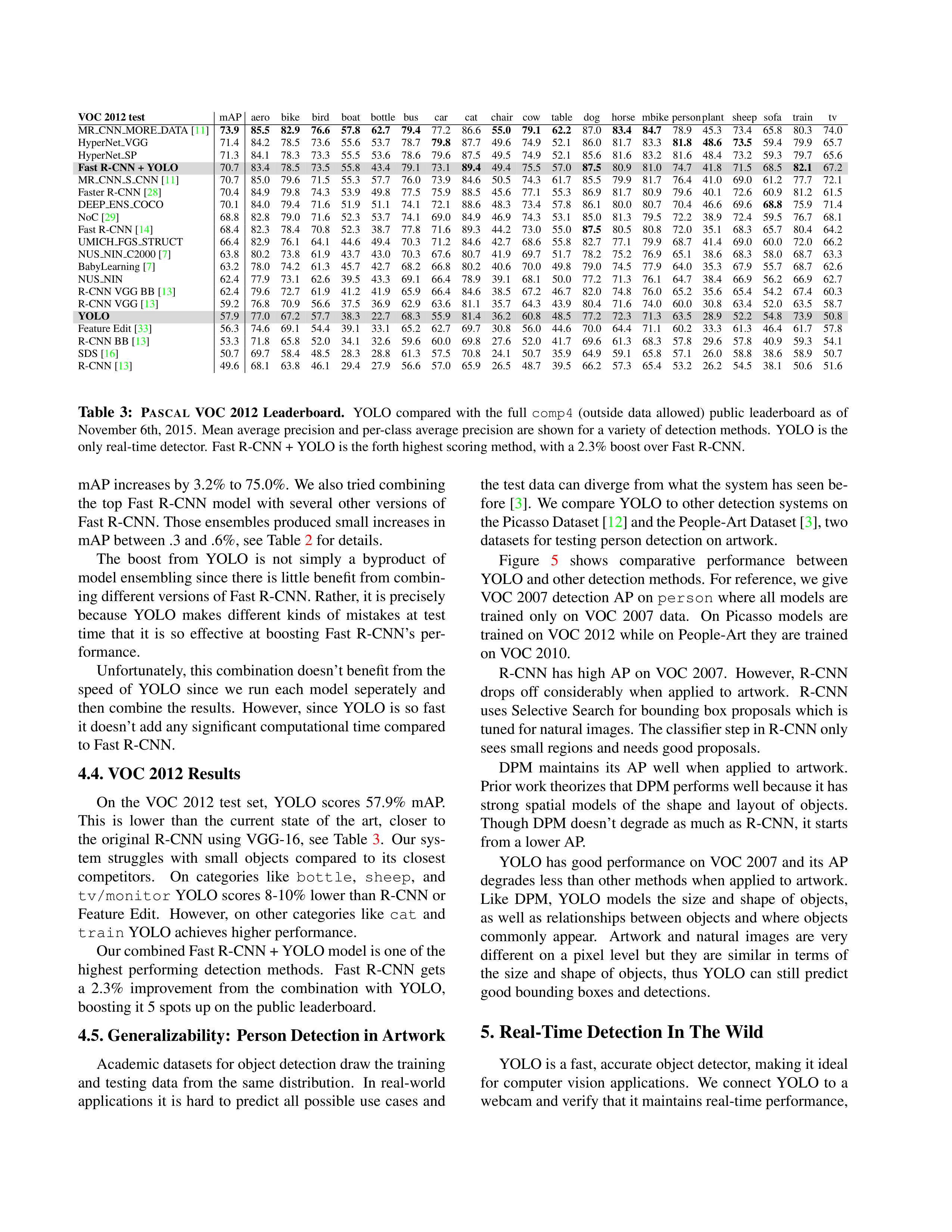
Table
3:
P
ASCAL
VOC
2012
Leaderboard.
YOLO
compared
with
the
full
comp4
(outside
data
allowed)
public
leaderboard
as
of
November 6th, 2015.
Mean average precision and per-class average precision are shown for a variety of detection methods.
YOLO is the
only real-time detector.
Fast R-CNN + YOLO is the forth highest scoring method, with a 2.3% boost over Fast R-CNN.
mAP increases by 3.2% to 75.0%.
We also tried combining
the
top
Fast
R-CNN
model
with
several
other
versions
of
Fast R-CNN. Those ensembles produced small increases in
mAP between .3 and .6%, see Table
2
for details.
The
boost
from
YOLO
is
not
simply
a
byproduct
of
model ensembling since there is little benefit from combin-
ing different versions of Fast R-CNN. Rather, it is precisely
because
YOLO
makes
different
kinds
of
mistakes
at
test
time
that
it
is
so
effective
at
boosting
Fast
R-CNN’s
per-
formance.
Unfortunately, this combination doesn’t benefit from the
speed
of
YOLO
since
we
run
each
model
seperately
and
then combine the results.
However,
since YOLO is so fast
it doesn’t add any significant computational time compared
to Fast R-CNN.
4.4. VOC 2012 Results
On
the
VOC
2012
test
set,
YOLO
scores
57.9%
mAP.
This
is
lower
than
the
current
state
of
the
art,
closer
to
the
original
R-CNN
using
VGG-16,
see
Table
3
.
Our
sys-
tem
struggles
with
small
objects
compared
to
its
closest
competitors.
On
categories
like
bottle
,
sheep
,
and
tv/monitor
YOLO scores 8-10% lower than R-CNN or
Feature
Edit.
However,
on
other
categories
like
cat
and
train
YOLO achieves higher performance.
Our combined Fast R-CNN + YOLO model is one of the
highest
performing
detection
methods.
Fast
R-CNN
gets
a
2.3%
improvement
from
the
combination
with
YOLO,
boosting it 5 spots up on the public leaderboard.
4.5. Generalizability:
Person Detection in Artwork
Academic datasets for object detection draw the training
and
testing
data
from
the
same
distribution.
In
real-world
applications
it
is
hard
to
predict
all
possible
use
cases
and
the test data can diverge from what the system has seen be-
fore [
3
].
We compare YOLO to other detection systems on
the Picasso Dataset [
12
] and the People-Art Dataset [
3
], two
datasets for testing person detection on artwork.
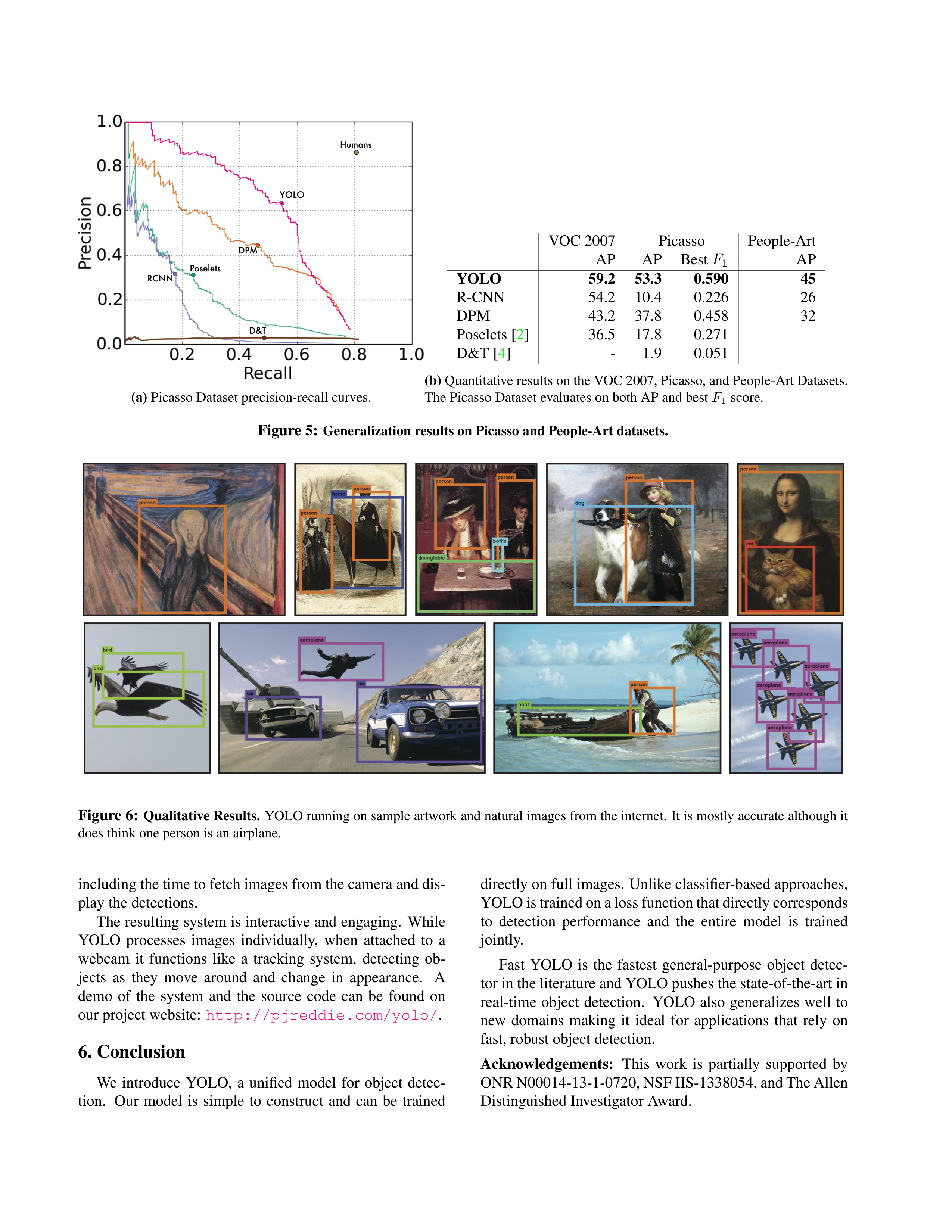
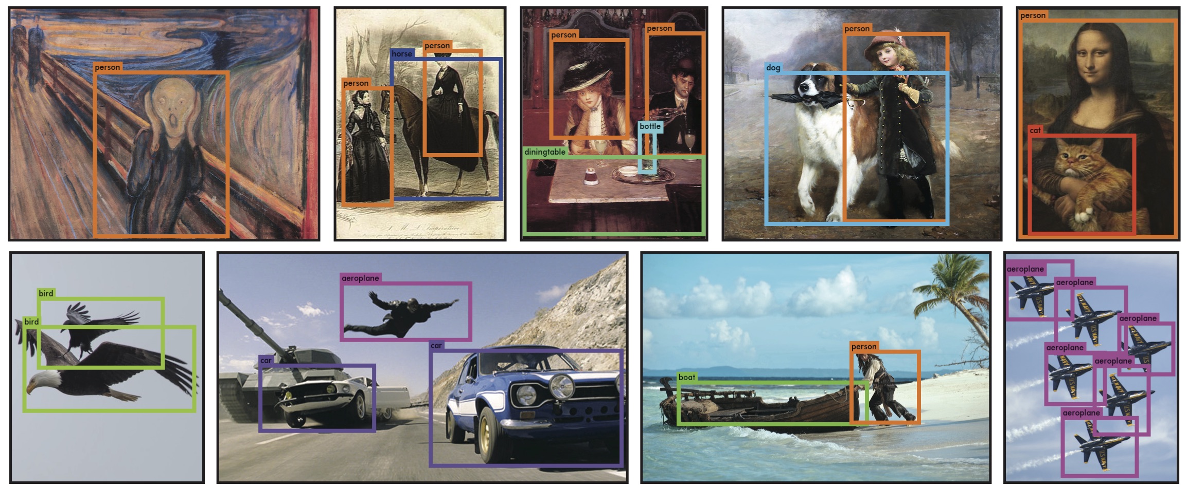
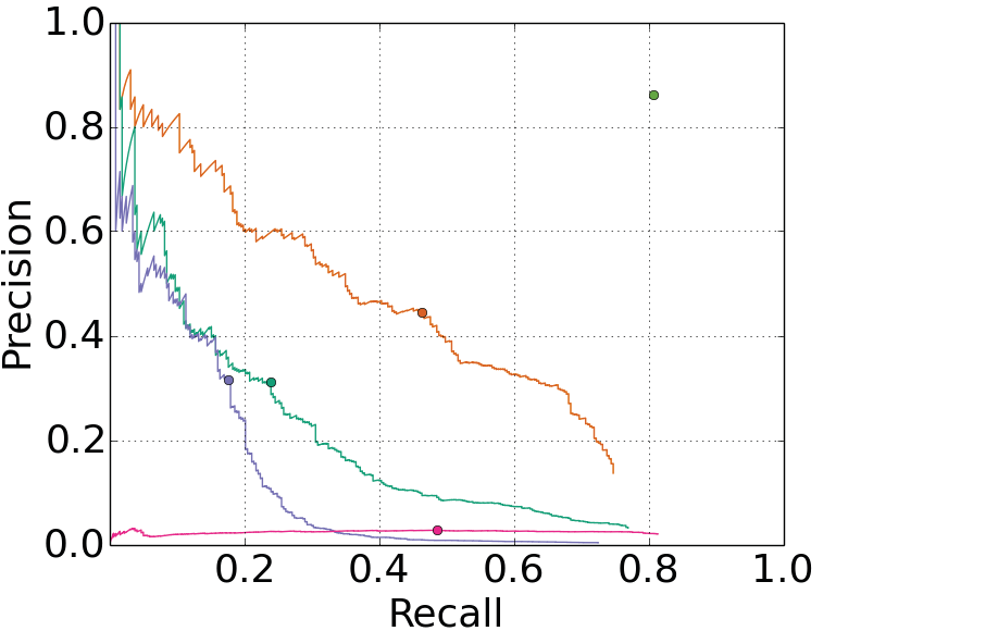
Figure
5
shows
comparative
performance
between
YOLO and other detection methods.
For reference, we give
VOC 2007 detection AP on
person
where all models are
trained
only
on
VOC
2007
data.
On
Picasso
models
are
trained on VOC 2012 while on People-Art they are trained
on VOC 2010.
R-CNN
has
high
AP
on
VOC
2007.
However,
R-CNN
drops
off
considerably
when
applied
to
artwork.
R-CNN
uses Selective Search for bounding box proposals which is
tuned for natural images.
The classifier step in R-CNN only
sees small regions and needs good proposals.
DPM
maintains
its
AP
well
when
applied
to
artwork.
Prior work theorizes that DPM performs well because it has
strong
spatial
models
of
the
shape
and
layout
of
objects.
Though DPM doesn’t degrade as much as R-CNN, it starts
from a lower AP.
YOLO has good performance on VOC 2007 and its AP
degrades less than other methods when applied to artwork.
Like
DPM,
YOLO
models
the
size
and
shape
of
objects,
as well as relationships between objects and where objects
commonly
appear.
Artwork
and
natural
images
are
very
different
on
a
pixel
level
but
they
are
similar
in
terms
of
the
size
and
shape
of
objects,
thus
YOLO
can
still
predict
good bounding boxes and detections.
5. Real-Time Detection In The Wild
YOLO is a fast, accurate object detector, making it ideal
for
computer
vision
applications.
We
connect
YOLO
to
a
webcam and verify that it maintains real-time performance,

Poselets
RCNN
D&T
Humans
DPM
YOLO
(a)
Picasso Dataset precision-recall curves.
VOC 2007
Picasso
People-Art
AP
AP
Best
F
1
AP
YOLO
59.2
53.3
0.590
45
R-CNN
54.2
10.4
0.226
26
DPM
43.2
37.8
0.458
32
Poselets [
2
]
36.5
17.8
0.271
D&T [
4
]
-
1.9
0.051
(b)
Quantitative results on the VOC 2007, Picasso, and People-Art Datasets.
The Picasso Dataset evaluates on both AP and best
F
1
score.
Figure 5:
Generalization results on Picasso and People-Art datasets.
Figure 6:
Qualitative Results.
YOLO running on sample artwork and natural images from the internet.
It is mostly accurate although it
does think one person is an airplane.
including the time to fetch images from the camera and dis-
play the detections.
The resulting system is interactive and engaging.
While
YOLO
processes
images
individually,
when
attached
to
a
webcam
it
functions
like
a
tracking
system,
detecting
ob-
jects
as
they
move
around
and
change
in
appearance.
A
demo
of
the
system
and
the
source
code
can
be
found
on
our project website:
http://pjreddie.com/yolo/
.
6. Conclusion
We
introduce
YOLO,
a
unified
model
for
object
detec-
tion.
Our
model
is
simple
to
construct
and
can
be
trained
directly on full images.
Unlike classifier-based approaches,
YOLO is trained on a loss function that directly corresponds
to
detection
performance
and
the
entire
model
is
trained
jointly.
Fast
YOLO
is
the
fastest
general-purpose
object
detec-
tor in the literature and YOLO pushes the state-of-the-art in
real-time
object
detection.
YOLO
also
generalizes
well
to
new
domains
making
it
ideal
for
applications
that
rely
on
fast, robust object detection.
Acknowledgements:
This
work
is
partially
supported
by
ONR N00014-13-1-0720, NSF IIS-1338054, and The Allen
Distinguished Investigator Award.
References
[1]
M. B. Blaschko and C. H. Lampert.
Learning to localize ob-
jects with structured output regression.
In
Computer Vision–
ECCV 2008
, pages 2–15. Springer, 2008.
4
[2]
L.
Bourdev
and
J.
Malik.
Poselets:
Body
part
detectors
trained
using
3d
human
pose
annotations.
In
International
Conference on Computer Vision (ICCV)
, 2009.
8
[3]
H.
Cai,
Q.
Wu,
T.
Corradi,
and
P.
Hall.
The
cross-
depiction
problem:
Computer
vision
algorithms
for
recog-
nising objects in artwork and in photographs.
arXiv preprint
arXiv:1505.00110
, 2015.
7
[4]
N. Dalal and B. Triggs.
Histograms of oriented gradients for
human detection.
In
Computer Vision and Pattern Recogni-
tion, 2005. CVPR 2005. IEEE Computer Society Conference
on
, volume 1, pages 886–893. IEEE, 2005.
4
,
8
[5]
T.
Dean,
M.
Ruzon,
M.
Segal,
J.
Shlens,
S.
Vijaya-
narasimhan,
J.
Yagnik,
et
al.
Fast,
accurate
detection
of
100,000
object
classes
on
a
single
machine.
In
Computer
Vision and Pattern Recognition (CVPR), 2013 IEEE Confer-
ence on
, pages 1814–1821. IEEE, 2013.
5
[6]
J.
Donahue,
Y.
Jia,
O.
Vinyals,
J.
Hoffman,
N.
Zhang,
E. Tzeng, and T. Darrell.
Decaf:
A deep convolutional acti-
vation feature for generic visual recognition.
arXiv preprint
arXiv:1310.1531
, 2013.
4
[7]
J.
Dong,
Q.
Chen,
S.
Yan,
and
A.
Yuille.
Towards
unified
object
detection
and
semantic
segmentation.
In
Computer
Vision–ECCV 2014
, pages 299–314. Springer, 2014.
7
[8]
D. Erhan, C. Szegedy, A. Toshev, and D. Anguelov.
Scalable
object
detection
using
deep
neural
networks.
In
Computer
Vision and Pattern Recognition (CVPR), 2014 IEEE Confer-
ence on
, pages 2155–2162. IEEE, 2014.
5
,
6
[9]
M.
Everingham,
S.
M.
A.
Eslami,
L.
Van
Gool,
C.
K.
I.
Williams, J. Winn, and A. Zisserman.
The pascal visual ob-
ject classes challenge: A retrospective.
International Journal
of Computer Vision
, 111(1):98–136, Jan. 2015.
2
[10]
P. F. Felzenszwalb, R. B. Girshick, D. McAllester, and D. Ra-
manan.
Object
detection
with
discriminatively
trained
part
based
models.
IEEE
Transactions
on
Pattern
Analysis
and
Machine Intelligence
, 32(9):1627–1645, 2010.
1
,
4
[11]
S. Gidaris and N. Komodakis.
Object detection via a multi-
region & semantic segmentation-aware CNN model.
CoRR
,
abs/1505.01749, 2015.
7
[12]
S. Ginosar, D. Haas, T. Brown, and J. Malik.
Detecting peo-
ple in cubist art. In
Computer Vision-ECCV 2014 Workshops
,
pages 101–116. Springer, 2014.
7
[13]
R. Girshick, J. Donahue, T. Darrell, and J. Malik.
Rich fea-
ture
hierarchies
for
accurate
object
detection
and
semantic
segmentation.
In
Computer Vision and Pattern Recognition
(CVPR),
2014
IEEE
Conference
on
,
pages
580–587.
IEEE,
2014.
1
,
4
,
7
[14]
R. B. Girshick.
Fast R-CNN.
CoRR
, abs/1504.08083, 2015.
2
,
5
,
6
,
7
[15]
S.
Gould,
T.
Gao,
and
D.
Koller.
Region-based
segmenta-
tion and object detection.
In
Advances in neural information
processing systems
, pages 655–663, 2009.
4
[16]
B. Hariharan, P. Arbel´aez, R. Girshick, and J. Malik.
Simul-
taneous
detection
and
segmentation.
In
Computer
Vision–
ECCV 2014
, pages 297–312. Springer, 2014.
7
[17]
K. He, X. Zhang, S. Ren, and J. Sun. Spatial pyramid pooling
in deep convolutional networks for visual recognition.
arXiv
preprint arXiv:1406.4729
, 2014.
5
[18]
G. E. Hinton, N. Srivastava, A. Krizhevsky, I. Sutskever, and
R.
R.
Salakhutdinov.
Improving
neural
networks
by
pre-
venting
co-adaptation
of
feature
detectors.
arXiv
preprint
arXiv:1207.0580
, 2012.
4
[19]
D. Hoiem, Y. Chodpathumwan, and Q. Dai. Diagnosing error
in object detectors.
In
Computer Vision–ECCV 2012
, pages
340–353. Springer, 2012.
6
[20]
K.
Lenc
and
A.
Vedaldi.
R-cnn
minus
r.
arXiv
preprint
arXiv:1506.06981
, 2015.
5
,
6
[21]
R. Lienhart and J. Maydt.
An extended set of haar-like fea-
tures for rapid object detection.
In
Image Processing. 2002.
Proceedings.
2002
International
Conference
on
,
volume
1,
pages I–900. IEEE, 2002.
4
[22]
M.
Lin,
Q.
Chen,
and
S.
Yan.
Network
in
network.
CoRR
,
abs/1312.4400, 2013.
2
[23]
D.
G.
Lowe.
Object
recognition
from
local
scale-invariant
features.
In
Computer
vision,
1999.
The
proceedings
of
the
seventh
IEEE
international
conference
on
,
volume
2,
pages
1150–1157. Ieee, 1999.
4
[24]
D.
Mishkin.
Models
accuracy
on
imagenet
2012
val.
https://github.com/BVLC/caffe/wiki/
Models-accuracy-on-ImageNet-2012-val
.
Ac-
cessed:
2015-10-2.
3
[25]
C.
P.
Papageorgiou,
M.
Oren,
and
T.
Poggio.
A
general
framework
for
object
detection.
In
Computer
vision,
1998.
sixth
international
conference
on
,
pages
555–562.
IEEE,
1998.
4
[26]
J.
Redmon.
Darknet:
Open
source
neural
networks
in
c.
http://pjreddie.com/darknet/
, 2013–2016.
3
[27]
J. Redmon and A. Angelova. Real-time grasp detection using
convolutional neural networks.
CoRR
, abs/1412.3128, 2014.
5
[28]
S.
Ren,
K.
He,
R.
Girshick,
and
J.
Sun.
Faster
r-cnn:
To-
wards
real-time
object
detection
with
region
proposal
net-
works.
arXiv preprint arXiv:1506.01497
, 2015.
5
,
6
,
7
[29]
S. Ren, K. He, R. B. Girshick, X. Zhang, and J. Sun.
Object
detection
networks
on
convolutional
feature
maps.
CoRR
,
abs/1504.06066, 2015.
3
,
7
[30]
O.
Russakovsky,
J.
Deng,
H.
Su,
J.
Krause,
S.
Satheesh,
S.
Ma,
Z.
Huang,
A.
Karpathy,
A.
Khosla,
M.
Bernstein,
A.
C.
Berg,
and
L.
Fei-Fei.
ImageNet
Large
Scale
Visual
Recognition
Challenge.
International
Journal
of
Computer
Vision (IJCV)
, 2015.
3
[31]
M.
A.
Sadeghi
and
D.
Forsyth.
30hz
object
detection
with
dpm
v5.
In
Computer
Vision–ECCV
2014
,
pages
65–79.
Springer, 2014.
5
,
6
[32]
P.
Sermanet,
D.
Eigen,
X.
Zhang,
M.
Mathieu,
R.
Fergus,
and
Y.
LeCun.
Overfeat:
Integrated
recognition,
localiza-
tion
and
detection
using
convolutional
networks.
CoRR
,
abs/1312.6229, 2013.
4
,
5
[33]
Z. Shen and X. Xue. Do more dropouts in pool5 feature maps
for better object detection.
arXiv preprint arXiv:1409.6911
,
2014.
7
[34]
C.
Szegedy,
W.
Liu,
Y.
Jia,
P.
Sermanet,
S.
Reed,
D.
Anguelov,
D.
Erhan,
V.
Vanhoucke,
and
A.
Rabinovich.
Going
deeper
with
convolutions.
CoRR
,
abs/1409.4842,
2014.
2
[35]
J.
R.
Uijlings,
K.
E.
van
de
Sande,
T.
Gevers,
and
A.
W.
Smeulders.
Selective
search
for
object
recognition.
Inter-
national journal of computer vision
, 104(2):154–171, 2013.
4
[36]
P.
Viola
and
M.
Jones.
Robust
real-time
object
detection.
International Journal of Computer Vision
, 4:34–47, 2001.
4
[37]
P.
Viola
and
M.
J.
Jones.
Robust
real-time
face
detection.
International
journal
of
computer
vision
,
57(2):137–154,
2004.
5
[38]
J. Yan, Z. Lei, L. Wen, and S. Z. Li.
The fastest deformable
part model for object detection.
In
Computer Vision and Pat-
tern Recognition (CVPR), 2014 IEEE Conference on
, pages
2497–2504. IEEE, 2014.
5
,
6
[39]
C. L. Zitnick and P. Doll´ar. Edge boxes: Locating object pro-
posals from edges.
In
Computer Vision–ECCV 2014
,
pages
391–405. Springer, 2014.
4