Published as a conference paper at ICLR 2018
G
RAPH
A
TTENTION
N
ETWORKS
Petar Veliˇckovi´c
∗
Department of Computer Science and Technology
University of Cambridge
petar.velickovic@cst.cam.ac.uk
Guillem Cucurull
∗
Centre de Visi´o per Computador, UAB
gcucurull@gmail.com
Arantxa Casanova
∗
Centre de Visi´o per Computador, UAB
ar.casanova.8@gmail.com
Adriana Romero
Montr´eal Institute for Learning Algorithms
adriana.romero.soriano@umontreal.ca
Pietro Li`o
Department of Computer Science and Technology
University of Cambridge
pietro.lio@cst.cam.ac.uk
Yoshua Bengio
Montr´eal Institute for Learning Algorithms
yoshua.umontreal@gmail.com
A
BSTRACT
We present graph attention networks (GATs), novel neural network architectures
that operate on graph-structured data, leveraging masked self-attentional layers to
address
the
shortcomings
of
prior
methods
based
on
graph
convolutions
or
their
approximations.
By
stacking
layers
in
which
nodes
are
able
to
attend
over
their
neighborhoods’
features,
we
enable
(implicitly)
specifying
different
weights
to
different nodes in a neighborhood, without requiring any kind of costly matrix op-
eration (such as inversion) or depending on knowing the graph structure upfront.
In this way, we address several key challenges of spectral-based graph neural net-
works simultaneously, and make our model readily applicable to inductive as well
as transductive problems. Our GAT models have achieved or matched state-of-the-
art
results
across
four
established
transductive
and
inductive
graph
benchmarks:
the
Cora
,
Citeseer
and
Pubmed
citation
network
datasets,
as
well
as
a
protein-
protein interaction
dataset (wherein test graphs remain unseen during training).
1
I
NTRODUCTION
Convolutional
Neural
Networks
(CNNs)
have
been
successfully
applied
to
tackle
problems
such
as
image
classification
(He
et
al.,
2016),
semantic
segmentation
(J´egou
et
al.,
2017)
or
machine
translation (Gehring et al., 2016), where the underlying data representation has a grid-like structure.
These architectures efficiently reuse their local filters, with learnable parameters, by applying them
to all the input positions.
However, many interesting tasks involve data that can not be represented in a grid-like structure and
that instead lies in an irregular domain.
This is the case of 3D meshes, social networks, telecommu-
nication networks, biological networks or brain connectomes.
Such data can usually be represented
in the form of graphs.
There have been several attempts in the literature to extend neural networks to deal with arbitrarily
structured graphs.
Early work used recursive neural networks to process data represented in graph
domains as directed acyclic graphs (Frasconi et al., 1998; Sperduti & Starita, 1997).
Graph Neural
Networks (GNNs) were introduced in Gori et al. (2005) and Scarselli et al. (2009) as a generalization
of recursive neural networks that can directly deal with a more general class of graphs, e.g.
cyclic,
directed
and
undirected
graphs.
GNNs
consist
of
an
iterative
process,
which
propagates
the
node
states
until
equilibrium;
followed
by
a
neural
network,
which
produces
an
output
for
each
node
∗
Work performed while the author was at the Montr´eal Institute of Learning Algorithms.
1
arXiv:1710.10903v3 [stat.ML] 4 Feb 2018
Published as a conference paper at ICLR 2018
based
on
its
state.
This
idea
was
adopted
and
improved
by
Li
et
al.
(2016),
which
propose
to
use
gated recurrent units (Cho et al., 2014) in the propagation step.
Nevertheless, there is an increasing interest in generalizing convolutions to the graph domain.
Ad-
vances in this direction are often categorized as spectral approaches and non-spectral approaches.
On one hand, spectral approaches work with a spectral representation of the graphs and have been
successfully
applied
in
the
context
of
node
classification.
In
Bruna
et
al.
(2014),
the
convolution
operation is defined in the Fourier domain by computing the eigendecomposition of the graph Lapla-
cian,
resulting
in
potentially
intense
computations and non-spatially localized filters.
These issues
were
addressed
by
subsequent
works.
Henaff
et
al.
(2015)
introduced
a
parameterization
of
the
spectral filters with smooth coefficients in order to make them spatially localized.
Later, Defferrard
et
al.
(2016)
proposed
to
approximate
the
filters
by
means
of
a
Chebyshev
expansion
of
the
graph
Laplacian,
removing
the
need
to
compute
the
eigenvectors
of
the
Laplacian
and
yielding
spatially
localized
filters.
Finally,
Kipf
&
Welling
(2017)
simplified
the
previous
method
by
restricting
the
filters to operate in a 1-step neighborhood around each node.
However, in all of the aforementioned
spectral
approaches,
the
learned
filters
depend
on
the
Laplacian
eigenbasis,
which
depends
on
the
graph structure.
Thus, a model trained on a specific structure can not be directly applied to a graph
with a different structure.
On
the
other
hand,
we
have
non-spectral
approaches
(Duvenaud
et
al.,
2015;
Atwood
&
Towsley,
2016; Hamilton et al., 2017), which define convolutions directly on the graph, operating on groups
of spatially close neighbors. One of the challenges of these approaches is to define an operator which
works
with
different
sized
neighborhoods
and
maintains
the
weight
sharing
property
of
CNNs.
In
some
cases,
this
requires
learning
a
specific
weight
matrix
for
each
node
degree
(Duvenaud
et
al.,
2015), using the powers of a transition matrix to define the neighborhood while learning weights for
each input channel and neighborhood degree (Atwood & Towsley, 2016), or extracting and normal-
izing neighborhoods containing a fixed number of nodes (Niepert et al., 2016).
Monti et al. (2016)
presented
mixture
model
CNNs
(MoNet),
a
spatial
approach
which
provides
a
unified
generaliza-
tion of CNN architectures to graphs.
More recently, Hamilton et al. (2017) introduced GraphSAGE,
a
method
for
computing
node
representations
in
an
inductive
manner.
This
technique
operates
by
sampling
a
fixed-size
neighborhood
of
each
node,
and
then
performing
a
specific
aggregator
over
it
(such
as
the
mean
over
all
the
sampled
neighbors’
feature
vectors,
or
the
result
of
feeding
them
through a recurrent neural network).
This approach has yielded impressive performance across sev-
eral large-scale inductive benchmarks.
Attention mechanisms have become almost a
de facto
standard in many sequence-based tasks (Bah-
danau
et
al.,
2015;
Gehring
et
al.,
2016).
One
of
the
benefits
of
attention
mechanisms
is
that
they
allow for dealing with variable sized inputs, focusing on the most relevant parts of the input to make
decisions.
When an attention mechanism is used to compute a representation of a single sequence,
it is commonly referred to as
self-attention
or
intra-attention
.
Together with Recurrent Neural Net-
works
(RNNs)
or
convolutions,
self-attention
has
proven
to
be
useful
for
tasks
such
as
machine
reading
(Cheng
et
al.,
2016)
and
learning
sentence
representations
(Lin
et
al.,
2017).
However,
Vaswani et al. (2017) showed that not only
self-attention
can improve a method based on RNNs or
convolutions, but also that it is sufficient for constructing a powerful model obtaining
state-of-the-art
performance on the machine translation task.
Inspired by this recent work, we introduce an attention-based architecture to perform node classifica-
tion of graph-structured data.
The idea is to compute the hidden representations of each node in the
graph, by attending over its neighbors, following a
self-attention
strategy.
The attention architecture
has several interesting properties:
(1) the operation is efficient, since it is parallelizable across node-
neighbor pairs; (2) it can be applied to graph nodes having different degrees by specifying arbitrary
weights
to
the
neighbors;
and
(3)
the
model
is
directly
applicable
to
inductive
learning
problems,
including
tasks
where
the
model
has
to
generalize
to
completely
unseen
graphs.
We
validate
the
proposed approach on four challenging benchmarks:
Cora
,
Citeseer
and
Pubmed
citation networks
as well as an inductive
protein-protein interaction
dataset, achieving or matching state-of-the-art re-
sults that highlight the potential of attention-based models when dealing with arbitrarily structured
graphs.
It is worth noting that, as Kipf & Welling (2017) and Atwood & Towsley (2016), our work can also
be reformulated as a particular instance of MoNet (Monti et al., 2016).
Moreover, our approach of
2
Published as a conference paper at ICLR 2018
sharing
a
neural
network
computation
across
edges
is
reminiscent
of
the
formulation
of
relational
networks
(Santoro
et
al.,
2017)
and
VAIN
(Hoshen,
2017),
wherein
relations
between
objects
or
agents
are
aggregated
pair-wise,
by
employing
a
shared
mechanism.
Similarly,
our
proposed
at-
tention
model can
be connected
to the works by Duan et al. (2017) and Denil et al. (2017),
which
use a neighborhood attention operation to compute attention coefficients between different objects
in
an
environment.
Other
related
approaches
include
locally
linear
embedding
(LLE)
(Roweis
&
Saul, 2000) and memory networks (Weston et al., 2014).
LLE selects a fixed number of neighbors
around each data point, and learns a weight coefficient for each neighbor to reconstruct each point
as a weighted sum of its neighbors.
A second optimization step extracts the point’s feature embed-
ding.
Memory
networks
also
share
some
connections
with
our
work,
in
particular,
if
we
interpret
the neighborhood of a node as the memory, which is used to compute the node features by attending
over its values, and then is updated by storing the new features in the same position.
2
GAT
ARCHITECTURE
In
this
section,
we
will
present
the
building
block layer
used
to
construct arbitrary
graph
attention
networks (through stacking this layer), and directly outline its theoretical and practical benefits and
limitations compared to prior work in the domain of neural graph processing.
2.1
G
RAPH
ATTENTIONAL
LAYER
We
will
start
by
describing
a
single
graph
attentional
layer
,
as
the
sole
layer
utilized
throughout
all of the GAT architectures used in our experiments.
The particular attentional setup utilized by us
closely follows the work of Bahdanau et al. (2015)—but the framework is agnostic to the particular
choice of attention mechanism.
The
input
to
our
layer
is
a
set
of
node
features,
h
=
{
⃗h
1
,⃗h
2
, . . . ,⃗h
N
}
,⃗h
i
∈
R
F
,
where
N
is
the
number of nodes, and
F
is the number of features in each node. The layer produces a new set of node
features (of potentially different cardinality
F
′
),
h
′
=
{
⃗h
′
1
,⃗h
′
2
, . . . ,⃗h
′
N
}
,⃗h
′
i
∈
R
F
′
, as its output.
In order
to
obtain
sufficient
expressive power to transform the input features into higher-level fea-
tures, at least one learnable linear transformation is required.
To that end, as an initial step, a shared
linear transformation, parametrized by a
weight matrix
,
W
∈
R
F
′
×
F
, is applied to every node.
We
then
perform
self-attention
on
the
nodes—a
shared
attentional
mechanism
a
:
R
F
′
×
R
F
′
→
R
computes
attention coefficients
e
ij
=
a
(
W
⃗h
i
,
W
⃗h
j
)
(1)
that indicate the
importance
of node
j
’s features to node
i
. In its most general formulation, the model
allows every node to attend on every other node,
dropping all structural information
.
We inject the
graph structure into the mechanism by performing
masked attention
—we only compute
e
ij
for nodes
j
∈N
i
, where
N
i
is some
neighborhood
of node
i
in the graph.
In all our experiments, these will
be exactly the first-order neighbors of
i
(including
i
).
To make coefficients easily comparable across
different nodes, we normalize them across all choices of
j
using the softmax function:
α
ij
= softmax
j
(
e
ij
) =
exp(
e
ij
)
P
k
∈N
i
exp(
e
ik
)
.
(2)
In
our
experiments,
the
attention
mechanism
a
is
a
single-layer
feedforward
neural
network,
parametrized by a weight vector
⃗
a
∈
R
2
F
′
, and applying the LeakyReLU nonlinearity (with negative
input
slope
α
=
0
.
2
).
Fully
expanded
out,
the
coefficients
computed
by
the
attention
mechanism
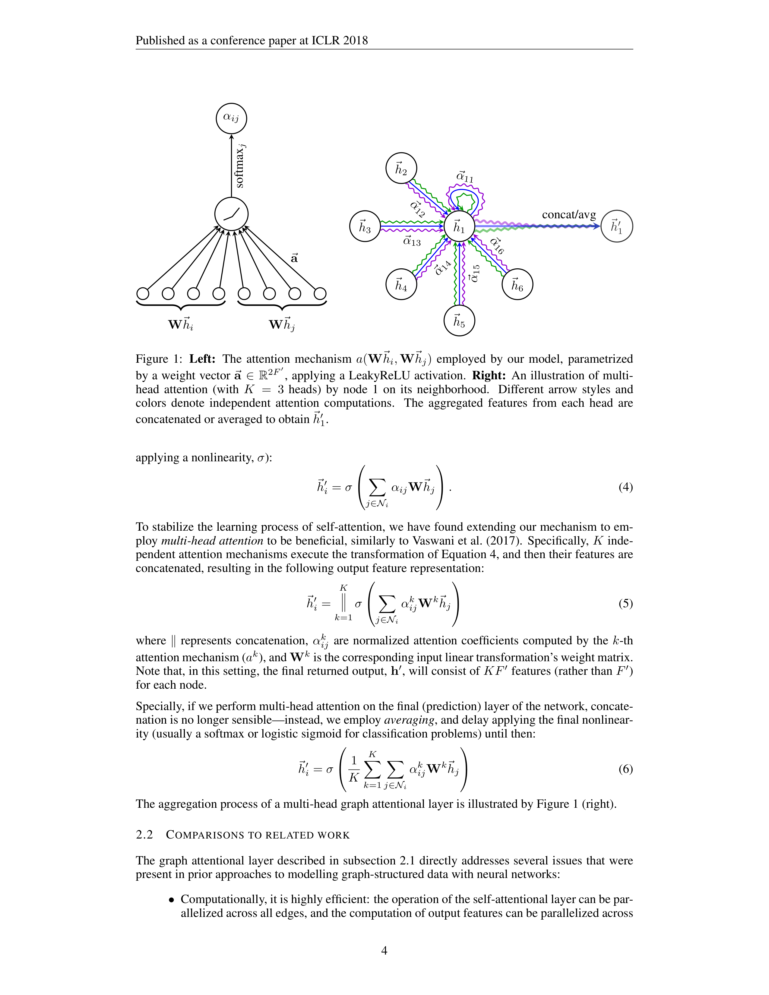
(illustrated by Figure 1 (left)) may then be expressed as:
α
ij
=
exp
LeakyReLU
a
T
[
W
⃗h
i
∥
W
⃗h
j
]
P
k
∈N
i
exp
LeakyReLU
a
T
[
W
⃗h
i
∥
W
⃗h
k
]
(3)
where
·
T
represents transposition and
∥
is the concatenation operation.
Once obtained, the normalized attention coefficients are used to compute a linear combination of the
features corresponding to them, to serve as the final output features for every node (after potentially
3
Published as a conference paper at ICLR 2018
α
ij
a
softmax
j
W
⃗h
i
W
⃗h
j
h
1
h
2
h
3
h
4
h
5
h
6
⃗
α
16
⃗
α
11
⃗
α
12
⃗
α
13
⃗
α
14
⃗
α
15
⃗
h
′
1
concat/avg
Figure
1:
Left:
The
attention
mechanism
a
(
W
⃗h
i
,
W
⃗h
j
)
employed
by
our
model,
parametrized
by
a
weight
vector
⃗
a
∈
R
2
F
′
,
applying
a
LeakyReLU
activation.
Right:
An
illustration
of
multi-
head
attention
(with
K
=
3
heads)
by
node
1
on
its
neighborhood.
Different
arrow
styles
and
colors
denote
independent
attention
computations.
The
aggregated
features
from
each
head
are
concatenated or averaged to obtain
⃗h
′
1
.
applying a nonlinearity,
σ
):
h
′
i
=
σ
X
j
∈N
i
α
ij
W
⃗h
j
.
(4)
To stabilize the learning process of self-attention, we have found extending our mechanism to em-
ploy
multi-head attention
to be beneficial, similarly to Vaswani et al. (2017).
Specifically,
K
inde-
pendent attention mechanisms execute the transformation of Equation 4, and then their features are
concatenated, resulting in the following output feature representation:
h
′
i
=
K
∥
k
=1
σ
X
j
∈N
i
α
k
ij
W
k
⃗h
j
(5)
where
∥
represents
concatenation,
α
k
ij
are
normalized
attention
coefficients
computed
by
the
k
-th
attention mechanism (
a
k
), and
W
k
is the corresponding input linear transformation’s weight matrix.
Note that, in this setting, the final returned output,
h
′
, will consist of
KF
′
features (rather than
F
′
)
for each node.
Specially, if we perform multi-head attention on the final (prediction) layer of the network, concate-
nation is no longer sensible—instead, we employ
averaging
, and delay applying the final nonlinear-
ity (usually a softmax or logistic sigmoid for classification problems) until then:
h
′
i
=
σ
1
K
K
X
k
=1
X
j
∈N
i
α
k
ij
W
k
⃗h
j
(6)
The aggregation process of a multi-head graph attentional layer is illustrated by Figure 1 (right).
2.2
C
OMPARISONS
TO
RELATED
WORK
The
graph
attentional
layer
described
in
subsection
2.1
directly
addresses
several
issues
that
were
present in prior approaches to modelling graph-structured data with neural networks:
•
Computationally, it is highly efficient: the operation of the self-attentional layer can be par-
allelized across all edges, and the computation of output features can be parallelized across
4
Published as a conference paper at ICLR 2018
all
nodes.
No
eigendecompositions
or
similar
costly
matrix
operations
are
required.
The
time complexity of a single GAT attention head computing
F
′
features may be expressed
as
O
(
|
V
|
FF
′
+
|
E
|
F
′
)
, where
F
is the number of input features, and
|
V
|
and
|
E
|
are the
numbers
of
nodes
and
edges
in
the
graph,
respectively.
This
complexity
is
on
par
with
the
baseline
methods
such
as
Graph
Convolutional
Networks
(GCNs)
(Kipf
&
Welling,
2017).
Applying
multi-head
attention
multiplies
the
storage
and
parameter
requirements
by a factor of
K
,
while the individual heads’ computations are fully independent and can
be parallelized.
•
As opposed to GCNs, our model allows for (implicitly) assigning
different importances
to
nodes of a same neighborhood, enabling a leap in model capacity.
Furthermore, analyzing
the
learned
attentional
weights
may
lead
to
benefits
in
interpretability,
as
was
the
case
in
the machine translation domain (e.g.
the qualitative analysis of Bahdanau et al. (2015)).
•
The attention mechanism is applied in a shared manner to all edges in the graph, and there-
fore it does not depend on upfront access to the global graph structure or (features of) all of
its nodes (a limitation of many prior techniques).
This has several desirable implications:
–
The graph is not required to be undirected (we may simply leave out computing
α
ij
if
edge
j
→
i
is not present).
–
It
makes
our
technique
directly
applicable
to
inductive
learning—including
tasks
where the model is evaluated on graphs that are
completely unseen
during training.
•
The
recently
published
inductive
method
of
Hamilton
et
al.
(2017)
samples
a
fixed-size
neighborhood
of
each
node,
in
order
to
keep
its
computational
footprint
consistent;
this
does
not
allow
it
access
to
the
entirety
of
the
neighborhood
while
performing
inference.
Moreover, this technique achieved some of its strongest results when an LSTM (Hochreiter
& Schmidhuber, 1997)-based neighborhood aggregator is used. This assumes the existence
of
a
consistent
sequential
node
ordering
across
neighborhoods,
and
the
authors
have
rec-
tified it by consistently feeding randomly-ordered sequences to the LSTM. Our technique
does not suffer from either of these issues—it works with the entirety of the neighborhood
(at
the
expense
of
a
variable
computational
footprint,
which
is
still
on-par
with
methods
like the GCN), and does not assume any ordering within it.
•
As
mentioned
in
Section
1,
GAT
can
be
reformulated
as
a
particular
instance
of
MoNet
(Monti
et
al.,
2016).
More
specifically,
setting
the
pseudo-coordinate
function
to
be
u
(
x, y
)
=
f
(
x
)
∥
f
(
y
)
,
where
f
(
x
)
represent
(potentially
MLP-transformed)
features
of
node
x
and
∥
is concatenation; and the weight function to be
w
j
(
u
) = softmax(MLP(
u
))
(with the softmax performed over the entire neighborhood of a node) would make MoNet’s
patch operator similar to ours.
Nevertheless, one should note that, in comparison to previ-
ously
considered
MoNet
instances,
our
model
uses
node
features
for
similarity
computa-
tions, rather than the node’s structural properties (which would assume knowing the graph
structure upfront).
We were able to produce a version of the GAT layer that leverages
sparse
matrix operations, reducing
the
storage
complexity
to
linear
in
the
number
of
nodes
and
edges
and
enabling
the
execution
of
GAT models on larger graph datasets.
However,
the tensor manipulation framework we used only
supports
sparse
matrix
multiplication
for
rank-2
tensors,
which
limits
the
batching
capabilities
of
the layer as it is currently implemented (especially for datasets with multiple graphs).
Appropriately
addressing this constraint is an important direction for future work.
Depending on the regularity of
the graph structure in place,
GPUs may not be able to offer major performance benefits compared
to
CPUs
in
these
sparse
scenarios.
It
should
also
be
noted
that
the
size
of
the
“receptive
field”
of
our model is upper-bounded by the depth of the network (similarly as for GCN and similar models).
Techniques
such
as
skip
connections
(He
et
al.,
2016)
could
be
readily
applied
for
appropriately
extending
the
depth,
however.
Lastly,
parallelization
across
all
the
graph
edges,
especially
in
a
distributed
manner,
may
involve
a
lot
of
redundant
computation,
as
the
neighborhoods
will
often
highly overlap in graphs of interest.
3
E
VALUATION
We
have
performed
comparative
evaluation
of
GAT
models
against
a
wide
variety
of
strong
base-
lines
and
previous
approaches,
on
four
established
graph-based
benchmark
tasks
(transductive
as
5
Published as a conference paper at ICLR 2018
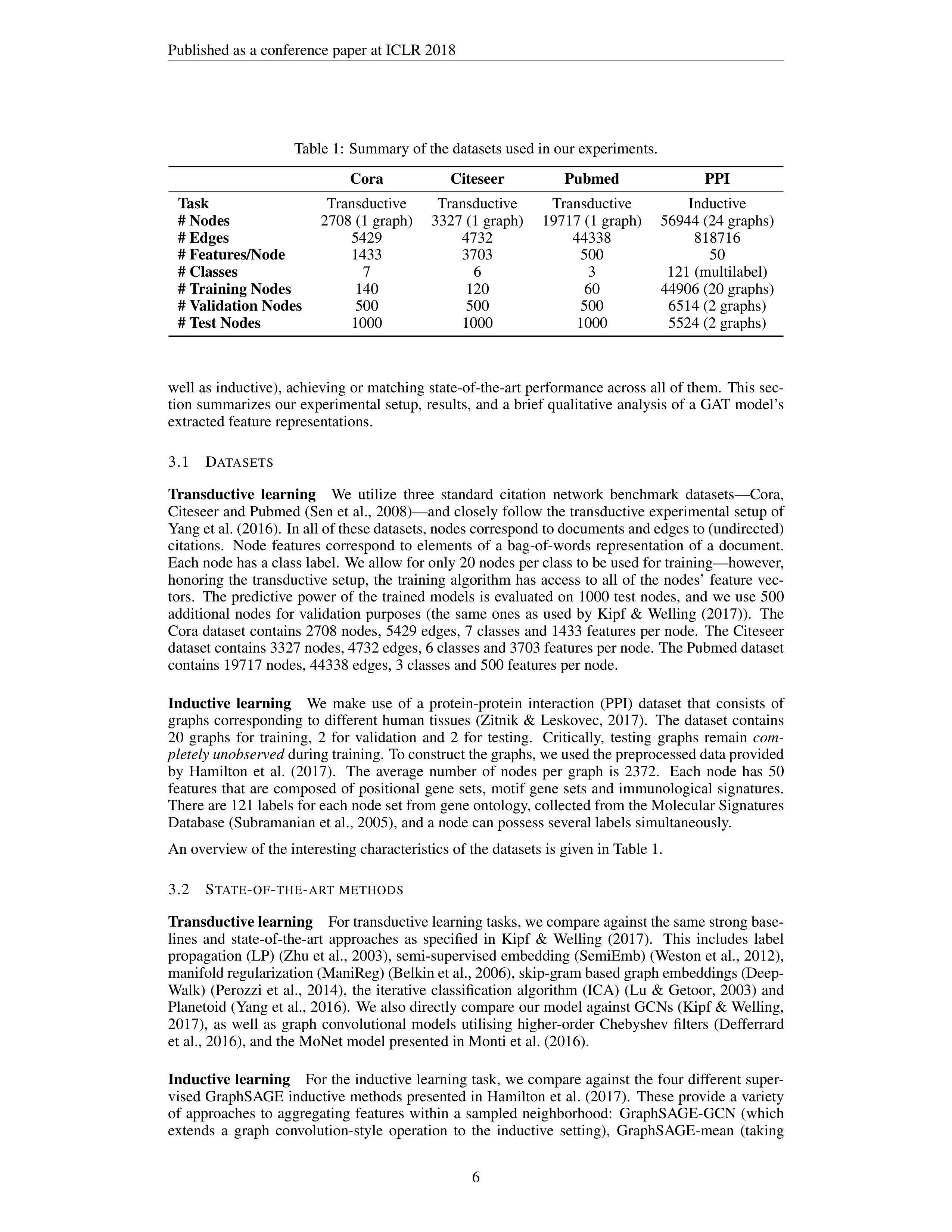
Table 1:
Summary of the datasets used in our experiments.
Cora
Citeseer
Pubmed
PPI
Task
Transductive
Transductive
Transductive
Inductive
# Nodes
2708 (1 graph)
3327 (1 graph)
19717 (1 graph)
56944 (24 graphs)
# Edges
5429
4732
44338
818716
# Features/Node
1433
3703
500
50
# Classes
7
6
3
121 (multilabel)
# Training Nodes
140
120
60
44906 (20 graphs)
# Validation Nodes
500
500
500
6514 (2 graphs)
# Test Nodes
1000
1000
1000
5524 (2 graphs)
well as inductive), achieving or matching state-of-the-art performance across all of them.
This sec-
tion summarizes our experimental setup, results,
and a brief qualitative analysis of a GAT model’s
extracted feature representations.
3.1
D
ATASETS
Transductive
learning
We
utilize
three
standard
citation
network
benchmark
datasets—Cora,
Citeseer and Pubmed (Sen et al., 2008)—and closely follow the transductive experimental setup of
Yang et al. (2016).
In all of these datasets, nodes correspond to documents and edges to (undirected)
citations.
Node
features
correspond
to
elements
of
a
bag-of-words
representation
of
a
document.
Each node has a class label.
We allow for only 20 nodes per class to be used for training—however,
honoring
the
transductive
setup,
the
training
algorithm
has
access
to
all
of
the
nodes’
feature
vec-
tors.
The
predictive
power
of
the
trained
models
is
evaluated
on
1000
test
nodes,
and
we
use
500
additional
nodes
for
validation
purposes
(the
same
ones
as
used
by
Kipf
&
Welling
(2017)).
The
Cora dataset contains 2708 nodes, 5429 edges, 7 classes and 1433 features per node.
The Citeseer
dataset contains 3327 nodes, 4732 edges, 6 classes and 3703 features per node.
The Pubmed dataset
contains 19717 nodes, 44338 edges, 3 classes and 500 features per node.
Inductive
learning
We
make
use
of
a
protein-protein
interaction
(PPI)
dataset
that
consists
of
graphs
corresponding
to
different
human
tissues
(Zitnik
&
Leskovec,
2017).
The
dataset
contains
20
graphs
for
training,
2
for
validation
and
2
for
testing.
Critically,
testing
graphs
remain
com-
pletely unobserved
during training.
To construct the graphs, we used the preprocessed data provided
by
Hamilton
et
al.
(2017).
The
average
number
of
nodes
per
graph
is
2372.
Each
node
has
50
features
that
are
composed
of
positional
gene
sets,
motif
gene
sets
and
immunological
signatures.
There are 121 labels for each node set from gene ontology, collected from the Molecular Signatures
Database (Subramanian et al., 2005), and a node can possess several labels simultaneously.
An overview of the interesting characteristics of the datasets is given in Table 1.
3.2
S
TATE
-
OF
-
THE
-
ART
METHODS
Transductive learning
For transductive learning tasks, we compare against the same strong base-
lines
and
state-of-the-art
approaches
as
specified
in
Kipf
&
Welling
(2017).
This
includes
label
propagation (LP) (Zhu et al., 2003), semi-supervised embedding (SemiEmb) (Weston et al., 2012),
manifold regularization (ManiReg) (Belkin et al., 2006), skip-gram based graph embeddings (Deep-
Walk)
(Perozzi
et
al.,
2014),
the
iterative
classification
algorithm
(ICA)
(Lu
&
Getoor,
2003)
and
Planetoid (Yang et al., 2016).
We also directly compare our model against GCNs (Kipf & Welling,
2017),
as
well
as
graph
convolutional
models
utilising
higher-order
Chebyshev
filters
(Defferrard
et al., 2016), and the MoNet model presented in Monti et al. (2016).
Inductive learning
For the inductive learning task,
we compare against the four different super-
vised GraphSAGE inductive methods presented in Hamilton et al. (2017).
These provide a variety
of
approaches
to
aggregating
features
within
a
sampled
neighborhood:
GraphSAGE-GCN
(which
extends
a
graph
convolution-style
operation
to
the
inductive
setting),
GraphSAGE-mean
(taking
6
Published as a conference paper at ICLR 2018
the
elementwise
mean
value
of
feature
vectors),
GraphSAGE-LSTM
(aggregating
by
feeding
the
neighborhood features into an LSTM) and GraphSAGE-pool (taking the elementwise maximization
operation
of
feature
vectors
transformed
by
a
shared
nonlinear
multilayer
perceptron).
The
other
transductive
approaches
are
either
completely
inappropriate
in
an
inductive
setting
or
assume
that
nodes
are
incrementally
added
to
a
single
graph,
making
them
unusable
for
the
setup
where
test
graphs are completely unseen during training (such as the PPI dataset).
Additionally, for both tasks we provide the performance of a per-node shared multilayer perceptron
(MLP) classifier (that does not incorporate graph structure at all).
3.3
E
XPERIMENTAL
SETUP
Transductive learning
For the transductive learning tasks, we apply a two-layer GAT model.
Its
architectural hyperparameters have been optimized on the Cora dataset and are then reused for Cite-
seer.
The first layer consists of
K
=
8
attention heads computing
F
′
=
8
features each (for a total
of 64 features), followed by an exponential linear unit (ELU) (Clevert et al., 2016) nonlinearity.
The
second
layer
is
used
for
classification:
a
single
attention
head
that
computes
C
features
(where
C
is the number of classes),
followed by a softmax activation.
For coping with the small training set
sizes, regularization is liberally applied within the model.
During training, we apply
L
2
regulariza-
tion
with
λ
=
0
.
0005
.
Furthermore,
dropout
(Srivastava
et
al.,
2014)
with
p
=
0
.
6
is
applied
to
both layers’ inputs, as well as
to the normalized attention coefficients
(critically, this means that at
each training iteration,
each node is exposed to a stochastically sampled neighborhood).
Similarly
as observed by Monti et al. (2016), we found that Pubmed’s training set size (60 examples) required
slight changes to the GAT architecture:
we have applied
K
=
8
output attention heads (instead of
one), and strengthened the
L
2
regularization to
λ
= 0
.
001
.
Otherwise, the architecture matches the
one used for Cora and Citeseer.
Inductive learning
For the inductive learning task, we apply a three-layer GAT model. Both of the
first two layers consist of
K
=
4
attention heads computing
F
′
=
256
features (for a total of 1024
features),
followed by an ELU nonlinearity.
The final layer is used for (multi-label) classification:
K
=
6
attention
heads
computing
121
features
each,
that
are
averaged
and
followed
by
a
logistic
sigmoid activation. The training sets for this task are sufficiently large and we found no need to apply
L
2
regularization or dropout—we have, however, successfully employed skip connections (He et al.,
2016) across the intermediate attentional layer. We utilize a batch size of 2 graphs during training. To
strictly evaluate the benefits of applying an attention mechanism in this setting (i.e.
comparing with
a
near
GCN-equivalent
model),
we
also
provide
the
results
when
a
constant
attention
mechanism
,
a
(
x, y
) = 1
, is used, with the same architecture—this will assign the same weight to every neighbor.
Both models are initialized using Glorot initialization (Glorot & Bengio, 2010) and trained to mini-
mize cross-entropy on the training nodes using the Adam SGD optimizer (Kingma & Ba, 2014) with
an
initial
learning
rate
of
0.01
for
Pubmed,
and
0.005
for
all
other
datasets.
In
both
cases
we
use
an
early
stopping
strategy
on
both
the
cross-entropy
loss
and
accuracy
(transductive)
or
micro-F
1
(inductive) score on the validation nodes, with a patience of 100 epochs
1
.
3.4
R
ESULTS
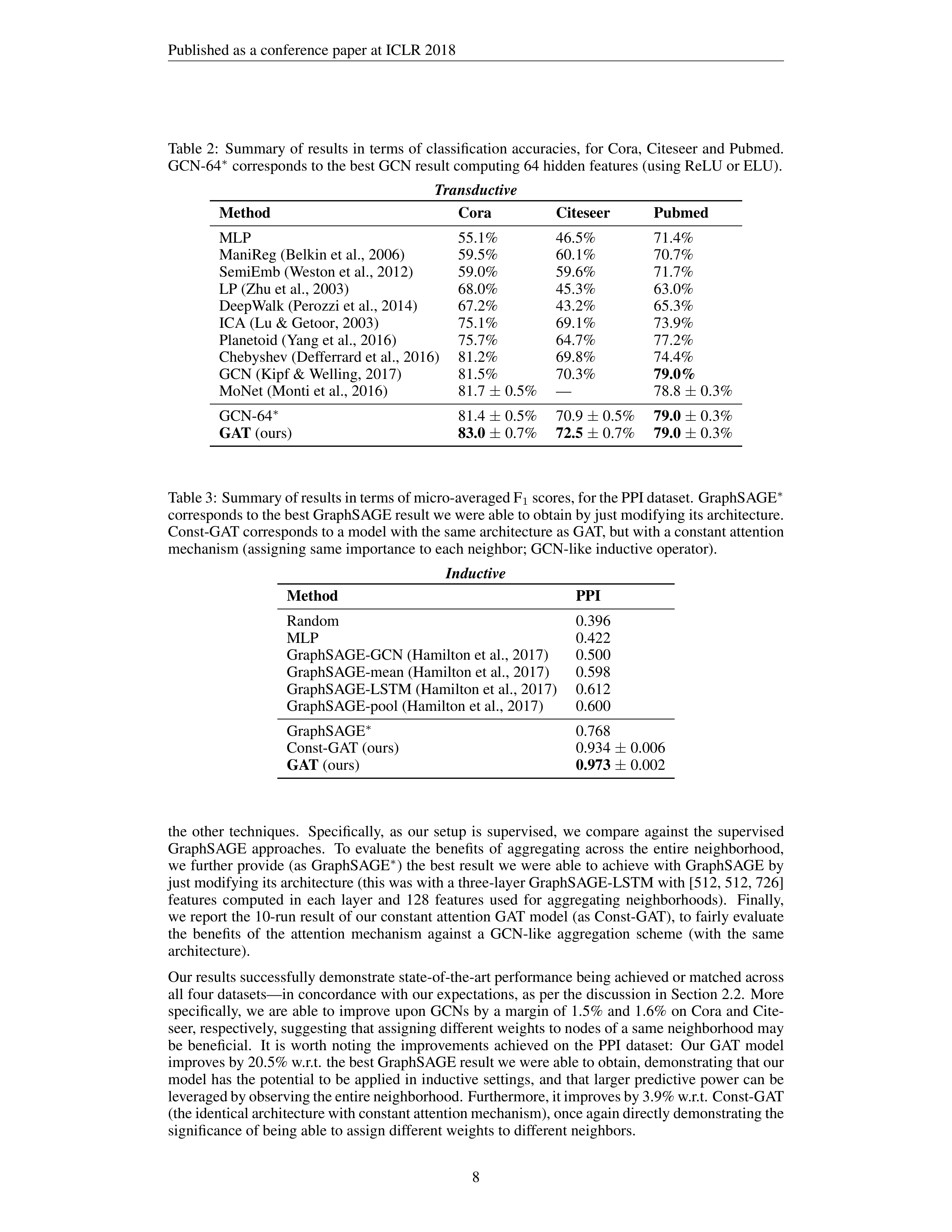
The results of our comparative evaluation experiments are summarized in Tables 2 and 3.
For the transductive tasks,
we report the mean classification accuracy (with standard deviation) on
the test nodes of our method after 100 runs, and reuse the metrics already reported in Kipf & Welling
(2017) and Monti et al. (2016) for state-of-the-art techniques.
Specifically, for the Chebyshev filter-
based approach (Defferrard et al., 2016), we provide the maximum reported performance for filters
of
orders
K
=
2
and
K
=
3
.
In
order
to
fairly
assess
the
benefits
of
the
attention
mechanism,
we further evaluate a GCN model that computes 64 hidden features, attempting both the ReLU and
ELU activation,
and reporting (as GCN-64
∗
) the better result after 100 runs (which was the ReLU
in all three cases).
For
the
inductive
task,
we
report
the
micro-averaged
F
1
score
on
the
nodes
of
the
two
unseen
test
graphs, averaged after 10 runs, and reuse the metrics already reported in Hamilton et al. (2017) for
1
Our implementation of the GAT layer may be found at:
https://github.com/PetarV-/GAT
.
7
Published as a conference paper at ICLR 2018
Table
2:
Summary
of
results
in
terms
of
classification
accuracies,
for
Cora,
Citeseer
and
Pubmed.
GCN-64
∗
corresponds to the best GCN result computing 64 hidden features (using ReLU or ELU).
Transductive
Method
Cora
Citeseer
Pubmed
MLP
55.1%
46.5%
71.4%
ManiReg (Belkin et al., 2006)
59.5%
60.1%
70.7%
SemiEmb (Weston et al., 2012)
59.0%
59.6%
71.7%
LP (Zhu et al., 2003)
68.0%
45.3%
63.0%
DeepWalk (Perozzi et al., 2014)
67.2%
43.2%
65.3%
ICA (Lu & Getoor, 2003)
75.1%
69.1%
73.9%
Planetoid (Yang et al., 2016)
75.7%
64.7%
77.2%
Chebyshev (Defferrard et al., 2016)
81.2%
69.8%
74.4%
GCN (Kipf & Welling, 2017)
81.5%
70.3%
79.0%
MoNet (Monti et al., 2016)
81.7
±
0.5%
—
78.8
±
0.3%
GCN-64
∗
81.4
±
0.5%
70.9
±
0.5%
79.0
±
0.3%
GAT
(ours)
83.0
±
0.7%
72.5
±
0.7%
79.0
±
0.3%
Table 3: Summary of results in terms of micro-averaged F
1
scores, for the PPI dataset. GraphSAGE
∗
corresponds to the best GraphSAGE result we were able to obtain by just modifying its architecture.
Const-GAT corresponds to a model with the same architecture as GAT, but with a constant attention
mechanism (assigning same importance to each neighbor; GCN-like inductive operator).
Inductive
Method
PPI
Random
0.396
MLP
0.422
GraphSAGE-GCN (Hamilton et al., 2017)
0.500
GraphSAGE-mean (Hamilton et al., 2017)
0.598
GraphSAGE-LSTM (Hamilton et al., 2017)
0.612
GraphSAGE-pool (Hamilton et al., 2017)
0.600
GraphSAGE
∗
0.768
Const-GAT (ours)
0.934
±
0.006
GAT
(ours)
0.973
±
0.002
the
other
techniques.
Specifically,
as
our
setup
is
supervised,
we
compare
against
the
supervised
GraphSAGE
approaches.
To
evaluate
the
benefits
of
aggregating
across
the
entire
neighborhood,
we further provide (as GraphSAGE
∗
) the best result we were able to achieve with GraphSAGE by
just modifying its architecture (this was with a three-layer GraphSAGE-LSTM with [512, 512, 726]
features
computed
in
each
layer
and
128
features
used
for
aggregating
neighborhoods).
Finally,
we report the 10-run result of our constant attention GAT model (as Const-GAT), to fairly evaluate
the
benefits
of
the
attention
mechanism
against
a
GCN-like
aggregation
scheme
(with
the
same
architecture).
Our results successfully demonstrate state-of-the-art performance being achieved or matched across
all four datasets—in concordance with our expectations, as per the discussion in Section 2.2.
More
specifically,
we are able to improve upon GCNs by a margin of 1.5% and 1.6% on Cora and Cite-
seer, respectively, suggesting that assigning different weights to nodes of a same neighborhood may
be
beneficial.
It
is
worth
noting
the
improvements
achieved
on
the
PPI
dataset:
Our
GAT
model
improves by 20.5% w.r.t.
the best GraphSAGE result we were able to obtain, demonstrating that our
model has the potential to be applied in inductive settings,
and that larger predictive power can be
leveraged by observing the entire neighborhood. Furthermore, it improves by 3.9% w.r.t. Const-GAT
(the identical architecture with constant attention mechanism), once again directly demonstrating the
significance of being able to assign different weights to different neighbors.
8
Published as a conference paper at ICLR 2018
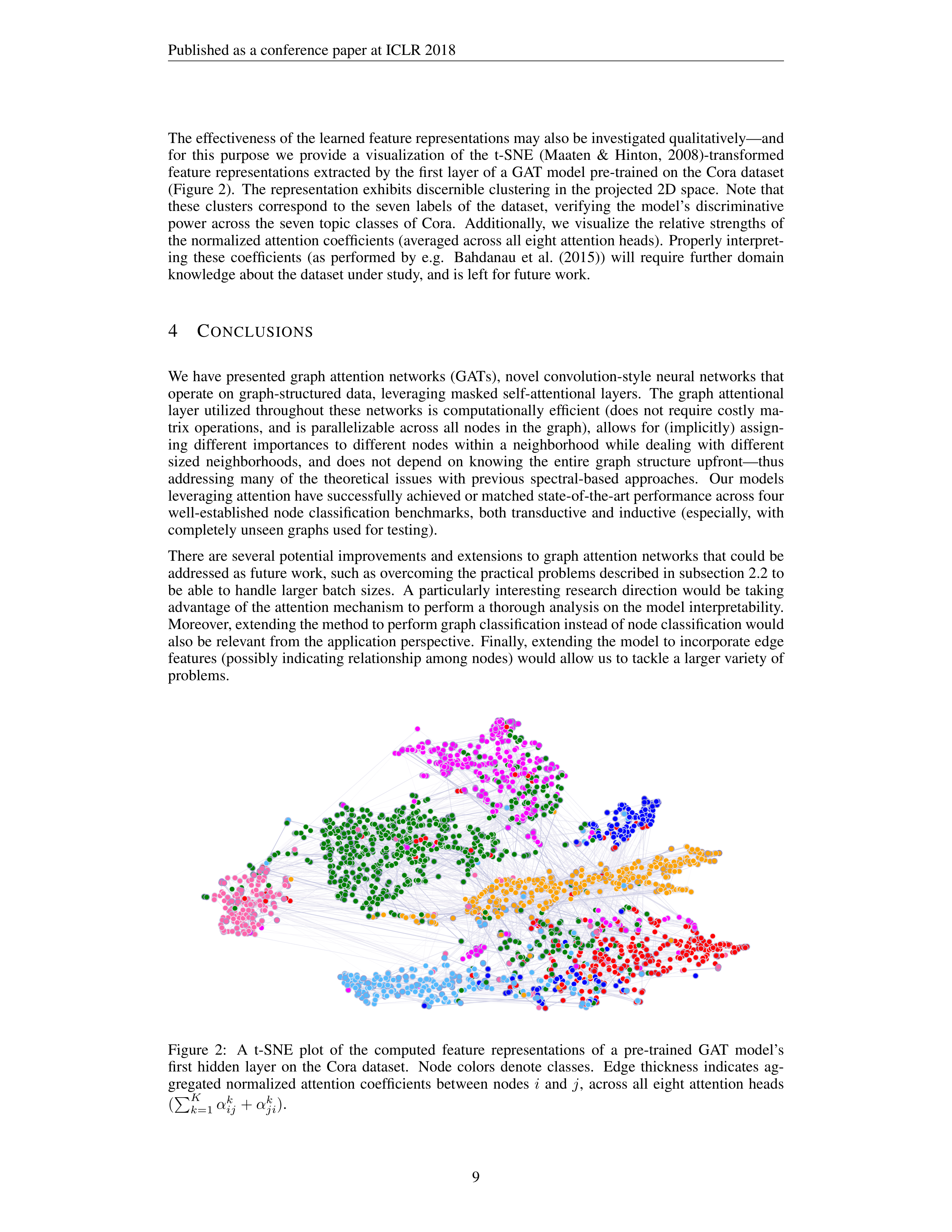
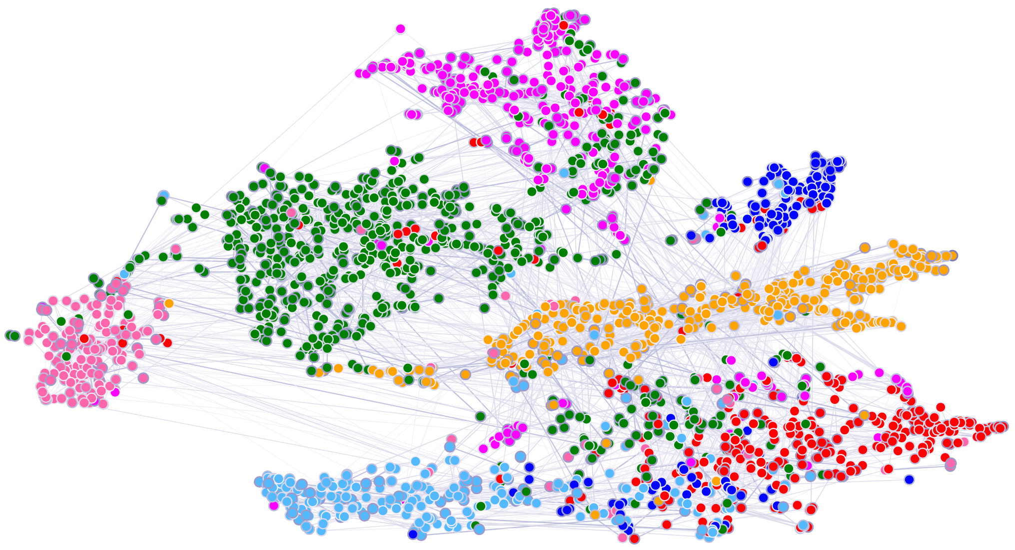
The effectiveness of the learned feature representations may also be investigated qualitatively—and
for
this
purpose
we
provide
a
visualization
of
the
t-SNE
(Maaten
&
Hinton,
2008)-transformed
feature representations extracted by the first layer of a GAT model pre-trained on the Cora dataset
(Figure 2).
The representation exhibits discernible clustering in the projected 2D space.
Note that
these
clusters
correspond
to
the
seven
labels
of
the
dataset,
verifying
the
model’s
discriminative
power
across
the
seven
topic
classes
of
Cora.
Additionally,
we
visualize
the
relative
strengths
of
the normalized attention coefficients (averaged across all eight attention heads).
Properly interpret-
ing
these
coefficients
(as
performed
by
e.g.
Bahdanau
et
al.
(2015))
will
require
further
domain
knowledge about the dataset under study, and is left for future work.
4
C
ONCLUSIONS
We have presented graph attention networks (GATs),
novel convolution-style neural networks that
operate
on
graph-structured
data,
leveraging
masked
self-attentional
layers.
The
graph
attentional
layer
utilized
throughout
these
networks
is
computationally
efficient
(does
not
require
costly
ma-
trix
operations,
and
is
parallelizable
across
all
nodes
in
the
graph),
allows
for
(implicitly)
assign-
ing
different
importances
to
different
nodes
within
a
neighborhood
while
dealing
with
different
sized
neighborhoods,
and
does
not
depend
on
knowing
the
entire
graph
structure
upfront—thus
addressing
many
of
the
theoretical
issues
with
previous
spectral-based
approaches.
Our
models
leveraging attention have successfully achieved or matched state-of-the-art performance across four
well-established
node
classification
benchmarks,
both
transductive
and
inductive
(especially,
with
completely unseen graphs used for testing).
There are several potential improvements and extensions to graph attention networks that could be
addressed as future work, such as overcoming the practical problems described in subsection 2.2 to
be
able
to
handle
larger
batch
sizes.
A
particularly
interesting
research
direction
would
be
taking
advantage of the attention mechanism to perform a thorough analysis on the model interpretability.
Moreover, extending the method to perform graph classification instead of node classification would
also be relevant from the application perspective.
Finally, extending the model to incorporate edge
features (possibly indicating relationship among nodes) would allow us to tackle a larger variety of
problems.
Figure
2:
A
t-SNE
plot
of
the
computed
feature
representations
of
a
pre-trained
GAT
model’s
first
hidden
layer
on
the
Cora
dataset.
Node
colors
denote
classes.
Edge
thickness
indicates
ag-
gregated
normalized
attention
coefficients
between
nodes
i
and
j
,
across
all
eight
attention
heads
(
P
K
k
=1
α
k
ij
+
α
k
ji
)
.
9
Published as a conference paper at ICLR 2018
A
CKNOWLEDGEMENTS
The authors would like to thank the developers of TensorFlow (Abadi et al., 2015).
PV and PL have
received
funding
from
the
European
Union’s
Horizon
2020
research
and
innovation
programme
PROPAG-AGEING under grant agreement No 634821.
We further acknowledge the support of the
following agencies for research funding and computing support:
CIFAR, Canada Research Chairs,
Compute
Canada
and
Calcul
Qu´ebec,
as
well
as
NVIDIA
for
the
generous
GPU
support.
Special
thanks to:
Benjamin Day and Fabian Jansen for kindly pointing out issues in a previous iteration of
the paper;
Michał Dro˙zd˙zal for useful discussions,
feedback and support;
and Ga´etan Marceau for
reviewing the paper prior to submission.
R
EFERENCES
Mart´ın Abadi, Ashish Agarwal, Paul Barham, Eugene Brevdo, Zhifeng Chen, Craig Citro, Greg S.
Corrado, Andy Davis, Jeffrey Dean, Matthieu Devin, Sanjay Ghemawat, Ian Goodfellow, Andrew
Harp, Geoffrey Irving, Michael Isard, Yangqing Jia, Rafal Jozefowicz, Lukasz Kaiser, Manjunath
Kudlur,
Josh
Levenberg,
Dan
Man´e,
Rajat
Monga,
Sherry
Moore,
Derek
Murray,
Chris
Olah,
Mike Schuster, Jonathon Shlens, Benoit Steiner, Ilya Sutskever, Kunal Talwar, Paul Tucker, Vin-
cent Vanhoucke, Vijay Vasudevan, Fernanda Vi´egas, Oriol Vinyals, Pete Warden, Martin Watten-
berg, Martin Wicke, Yuan Yu, and Xiaoqiang Zheng.
TensorFlow:
Large-scale machine learning
on heterogeneous systems, 2015.
URL
https://www.tensorflow.org/
.
Software avail-
able from tensorflow.org.
James Atwood and Don Towsley.
Diffusion-convolutional neural networks.
In
Advances in Neural
Information Processing Systems
, pp. 1993–2001, 2016.
Dzmitry
Bahdanau,
Kyunghyun
Cho,
and
Yoshua
Bengio.
Neural
machine
translation
by
jointly
learning
to
align
and
translate.
International
Conference
on
Learning
Representations
(ICLR)
,
2015.
Mikhail Belkin, Partha Niyogi, and Vikas Sindhwani.
Manifold regularization:
A geometric frame-
work for learning from labeled and unlabeled examples.
Journal of machine learning research
, 7
(Nov):2399–2434, 2006.
Joan
Bruna,
Wojciech
Zaremba,
Arthur
Szlam,
and
Yann
LeCun.
Spectral
networks
and
locally
connected
networks
on
graphs.
International
Conference
on
Learning
Representations
(ICLR)
,
2014.
Jianpeng
Cheng,
Li
Dong,
and
Mirella
Lapata.
Long
short-term
memory-networks
for
machine
reading.
arXiv preprint arXiv:1601.06733
, 2016.
Kyunghyun Cho, Bart Van Merri¨enboer, Caglar Gulcehre, Dzmitry Bahdanau, Fethi Bougares, Hol-
ger
Schwenk,
and
Yoshua
Bengio.
Learning
phrase
representations
using
rnn
encoder-decoder
for statistical machine translation.
arXiv preprint arXiv:1406.1078
, 2014.
Djork-Arn´e
Clevert,
Thomas
Unterthiner,
and
Sepp
Hochreiter.
Fast
and
accurate
deep
network
learning by exponential linear units (elus).
International Conference on Learning Representations
(ICLR)
, 2016.
Micha¨el
Defferrard,
Xavier
Bresson,
and
Pierre
Vandergheynst.
Convolutional
neural
networks
on
graphs
with
fast
localized
spectral
filtering.
In
Advances
in
Neural
Information
Processing
Systems
, pp. 3844–3852, 2016.
Misha Denil, Sergio G´omez Colmenarejo, Serkan Cabi, David Saxton, and Nando de Freitas.
Pro-
grammable agents.
arXiv preprint arXiv:1706.06383
, 2017.
Yan
Duan,
Marcin
Andrychowicz,
Bradly
Stadie,
Jonathan
Ho,
Jonas
Schneider,
Ilya
Sutskever,
Pieter
Abbeel,
and
Wojciech
Zaremba.
One-shot
imitation
learning.
arXiv
preprint
arXiv:1703.07326
, 2017.
David K Duvenaud, Dougal Maclaurin, Jorge Iparraguirre, Rafael Bombarell, Timothy Hirzel, Al´an
Aspuru-Guzik,
and
Ryan
P
Adams.
Convolutional
networks
on
graphs
for
learning
molecular
fingerprints.
In
Advances in neural information processing systems
, pp. 2224–2232, 2015.
10
Published as a conference paper at ICLR 2018
Paolo Frasconi, Marco Gori, and Alessandro Sperduti. A general framework for adaptive processing
of data structures.
IEEE transactions on Neural Networks
, 9(5):768–786, 1998.
Jonas
Gehring,
Michael
Auli,
David
Grangier,
and
Yann
N.
Dauphin.
A
convolutional
encoder
model
for
neural
machine
translation.
CoRR
,
abs/1611.02344,
2016.
URL
http://arxiv.
org/abs/1611.02344
.
Xavier Glorot and Yoshua Bengio.
Understanding the difficulty of training deep feedforward neural
networks.
In
Proceedings
of
the
Thirteenth
International
Conference
on
Artificial
Intelligence
and Statistics
, pp. 249–256, 2010.
Marco Gori, Gabriele Monfardini, and Franco Scarselli. A new model for learning in graph domains.
In
IEEE International Joint Conference on Neural Networks
, pp. 729734, 2005.
William
L
Hamilton,
Rex
Ying,
and
Jure
Leskovec.
Inductive
representation
learning
on
large
graphs.
Neural Information Processing Systems (NIPS)
, 2017.
Kaiming He, Xiangyu Zhang, Shaoqing Ren, and Jian Sun.
Deep residual learning for image recog-
nition.
In
Proceedings
of
the
IEEE
conference
on
computer
vision
and
pattern
recognition
,
pp.
770–778, 2016.
Mikael
Henaff,
Joan
Bruna,
and
Yann
LeCun.
Deep
convolutional
networks
on
graph-structured
data.
arXiv preprint arXiv:1506.05163
, 2015.
Sepp
Hochreiter
and
J¨urgen
Schmidhuber.
Long
short-term
memory.
Neural
computation
,
9(8):
1735–1780, 1997.
Yedid
Hoshen.
Vain:
Attentional
multi-agent
predictive
modeling.
In
I.
Guyon,
U.
V.
Luxburg,
S.
Bengio,
H.
Wallach,
R.
Fergus,
S.
Vishwanathan,
and
R.
Gar-
nett
(eds.),
Advances
in
Neural
Information
Processing
Systems
30
,
pp.
2698–
2708.
Curran
Associates,
Inc.,
2017.
URL
http://papers.nips.cc/paper/
6863-vain-attentional-multi-agent-predictive-modeling.pdf
.
Simon
J´egou,
Michal
Drozdzal,
David
V´azquez,
Adriana
Romero,
and
Yoshua
Bengio.
The
one
hundred layers tiramisu:
Fully convolutional densenets for semantic segmentation.
In
Workshop
on Computer Vision in Vehicle Technology CVPRW
, 2017.
Diederik
Kingma
and
Jimmy
Ba.
Adam:
A
method
for
stochastic
optimization.
arXiv
preprint
arXiv:1412.6980
, 2014.
Thomas
N
Kipf
and
Max
Welling.
Semi-supervised
classification
with
graph
convolutional
net-
works.
International Conference on Learning Representations (ICLR)
, 2017.
Yujia
Li,
Daniel
Tarlow,
Marc
Brockschmidt,
and
Richard
Zemel.
Gated
graph
sequence
neural
networks.
International Conference on Learning Representations (ICLR)
, 2016.
Zhouhan
Lin,
Minwei
Feng,
Cicero
Nogueira
dos
Santos,
Mo
Yu,
Bing
Xiang,
Bowen
Zhou,
and
Yoshua
Bengio.
A
structured
self-attentive
sentence
embedding.
arXiv
preprint
arXiv:1703.03130
, 2017.
Qing
Lu
and
Lise
Getoor.
Link-based
classification.
In
Proceedings
of
the
20th
International
Conference on Machine Learning (ICML-03)
, pp. 496–503, 2003.
Laurens
van
der
Maaten
and
Geoffrey
Hinton.
Visualizing
data
using
t-sne.
Journal
of
Machine
Learning Research
, 9(Nov):2579–2605, 2008.
Federico Monti, Davide Boscaini, Jonathan Masci, Emanuele Rodol`a, Jan Svoboda, and Michael M
Bronstein.
Geometric
deep learning on graphs and manifolds using mixture model cnns.
arXiv
preprint arXiv:1611.08402
, 2016.
Mathias
Niepert,
Mohamed
Ahmed,
and
Konstantin
Kutzkov.
Learning
convolutional
neural
net-
works
for
graphs.
In
Proceedings
of
The
33rd
International
Conference
on
Machine
Learning
,
volume 48, pp. 2014–2023, 2016.
11
Published as a conference paper at ICLR 2018
Bryan
Perozzi,
Rami
Al-Rfou,
and
Steven
Skiena.
Deepwalk:
Online
learning
of
social
repre-
sentations.
In
Proceedings
of
the
20th
ACM
SIGKDD
international
conference
on
Knowledge
discovery and data mining
, pp. 701–710. ACM, 2014.
Sam T. Roweis and Lawrence K. Saul.
Nonlinear dimensionality reduction by locally linear embed-
ding.
Science
, 290:2323–2326, 2000.
Adam
Santoro,
David
Raposo,
David
GT
Barrett,
Mateusz
Malinowski,
Razvan
Pascanu,
Peter
Battaglia, and Timothy Lillicrap.
A simple neural network module for relational reasoning.
arXiv
preprint arXiv:1706.01427
, 2017.
Franco
Scarselli,
Marco
Gori,
Ah
Chung
Tsoi,
Markus
Hagenbuchner,
and
Gabriele
Monfardini.
The graph neural network model.
IEEE Transactions on Neural Networks
, 20(1):61–80, 2009.
Prithviraj Sen, Galileo Namata, Mustafa Bilgic, Lise Getoor, Brian Galligher, and Tina Eliassi-Rad.
Collective classification in network data.
AI magazine
, 29(3):93, 2008.
A.
Sperduti
and
A.
Starita.
Supervised
neural
networks
for
the
classification
of
structures.
Trans.
Neur. Netw.
, 8(3):714–735, May 1997.
ISSN 1045-9227.
doi:
10.1109/72.572108.
Nitish Srivastava,
Geoffrey E Hinton,
Alex Krizhevsky,
Ilya Sutskever,
and Ruslan Salakhutdinov.
Dropout:
a simple way to prevent neural networks from overfitting.
Journal of machine learning
research
, 15(1):1929–1958, 2014.
Aravind
Subramanian,
Pablo
Tamayo,
Vamsi
K
Mootha,
Sayan
Mukherjee,
Benjamin
L
Ebert,
Michael
A
Gillette,
Amanda
Paulovich,
Scott
L
Pomeroy,
Todd
R
Golub,
Eric
S
Lander,
et
al.
Gene set enrichment analysis: a knowledge-based approach for interpreting genome-wide expres-
sion profiles.
Proceedings of the National Academy of Sciences
, 102(43):15545–15550, 2005.
Ashish
Vaswani,
Noam
Shazeer,
Niki
Parmar,
Jakob
Uszkoreit,
Llion
Jones,
Aidan
N
Gomez,
Lukasz Kaiser, and Illia Polosukhin.
Attention is all you need.
arXiv preprint arXiv:1706.03762
,
2017.
Jason
Weston,
Fr´ed´eric
Ratle,
Hossein
Mobahi,
and
Ronan
Collobert.
Deep
learning
via
semi-
supervised embedding.
In
Neural Networks:
Tricks of the Trade
, pp. 639–655. Springer, 2012.
Jason Weston, Sumit Chopra, and Antoine Bordes.
Memory networks.
CoRR
, abs/1410.3916, 2014.
URL
http://arxiv.org/abs/1410.3916
.
Zhilin
Yang,
William
Cohen,
and
Ruslan
Salakhudinov.
Revisiting
semi-supervised
learning
with
graph embeddings.
In
International Conference on Machine Learning
, pp. 40–48, 2016.
Xiaojin
Zhu,
Zoubin
Ghahramani,
and
John
D
Lafferty.
Semi-supervised
learning
using
gaussian
fields and harmonic functions.
In
Proceedings of the 20th International conference on Machine
learning (ICML-03)
, pp. 912–919, 2003.
Marinka
Zitnik
and
Jure
Leskovec.
Predicting
multicellular
function
through
multi-layer
tissue
networks.
Bioinformatics
, 33(14):i190–i198, 2017.
12